

Guest blogger James Dean of Plastometrex and Double Precision Consultancy (one of our COMSOL Certified Consultants) discusses using finite element modeling (FEM) to understand hardness numbers, and how simulation applications and COMSOL Compiler™ have enabled Plastometrex to create a brand new product that enables stress-strain curves to be obtained from indentation test data…
Hardness tests of various types have been in use for many decades. They are quick and easy to carry out. The volume of material being tested is fairly small, so it’s possible to map the hardness number across surfaces, exploring local variations, and to obtain values from thin surface layers and coatings. The problem with hardness is that it’s not a well-defined property. The number obtained from a given sample varies between types of test, and also for the same test with different conditions. Similar hardness numbers are obtained from materials exhibiting a wide range of yielding and work hardening characteristics. The reasons for this are well understood and the effect is illustrated here using the COMSOL Multiphysics® software.
Concept of a Hardness Number (Obtained by Indentation)
Hardness is a measure of the resistance that a material offers to plastic deformation. It’s of interest to have information, not only about the yield stress but also about the subsequent work hardening characteristics. The hardness number provides a yardstick that incorporates both, although not in a well-defined manner. In view of the complexity of what it represents, it’s unsurprising that hardness is not a simple, well-defined parameter and there are several different hardness measurement schemes, each giving different numbers. The idea, however, is the same for all of these schemes. A specified load is applied to an indenter, which penetrates into the specimen, causing plastic deformation and leaving a permanent depression. A hardness number can be obtained in several ways, but in most cases, this is either via measurement of the indent lateral size (diameter) or of the penetration depth.
Hardness is commonly defined as the force (load) divided by the area of contact between indenter and specimen. This ratio has dimensions of stress, although it is usually quoted as simply a number (with units of kgf mm-2). In any event, this stress level bears no simple relation to the stress-strain curve of the material, or indeed to the stress field created in the sample. Different regions of the specimen will have been subjected to different plastic strain levels, ranging from zero (at the edge of the plastic zone) to perhaps several tens of percent (close to the indenter). Even this maximum strain level is not well defined, since it depends on the indenter shape, the applied load, and the plasticity characteristics. While the stress-strain relationship of the material does dictate the indent dimensions (for a given indenter shape and load), inferring the former from the latter is not straightforward and no attempt is made to do this in conventional hardness testing.
Brinell and Vickers Tests
The Brinell test, developed in 1900, involves pushing a 10 mm diameter hard sphere into the sample, using a 3000 kg (~30 kN) load. The Brinell hardness number is given by
(1)
where F is the applied load (in kgf), D (mm) is the diameter of the indenter, and d (mm) is the diameter (in projection view) of the indent. This formula corresponds to the load divided by the contact area. Such formulas are based on a simple geometric approach. Elastic recovery of the specimen is neglected. Furthermore, in practice, there may be “pileup” or “sink-in” around the indent, such that the true area of contact differs from that obtained from idealized geometry (and also making accurate measurement of the diameter difficult).
The Vickers test was developed in 1924 by Smith and Sandland (at Vickers Ltd.) A key objective was to reduce the load requirements of earlier tests. Changing the indenter from a relatively large sphere to a smaller and “sharper” shape allowed a lower load (that could be created with a dead weight) to be used. Several such weights are usually provided inside the machine, ranging from below 1 kg up to around 50 kg, depending on the model. The (diamond) indenter is a right pyramid with a square base and an angle of 136˚ between opposite faces. The (sharp) edges promote penetration and the lines that they produce in the indent facilitate measurement of its size.
The indent diameter, d, is measured in projection (as for the Brinell test). The value of HV (load divided by contact area) is given by
(2)
A simple calculation, similar to that for the Brinell test, thus allows the hardness number to be obtained from the measured value of d. As with the Brinell test, elastic recovery of the specimen, and “pileup” or “sink-in” around the indent, are neglected.
The Vickers test is widely used. In fact, HV is the most commonly quoted of the hardness numbers, partly because by varying the load, it can be applied to a wide range of metals, thin sections, surface layers, etc. Fig. 1 shows a typical set of values (Ref. 1), covering various alloys. These were obtained via a careful set of measurements on indent dimensions in particular samples. These data do serve to illustrate typical ranges, although the exact numerical values should, to say the least, be treated cautiously.
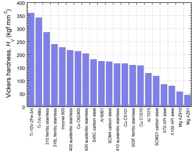
Figure 1. Data (Ref. 1) for the Vickers hardness of a range of alloys.
The stress acting on the contact area (in MPa) is obtained by multiplying this hardness number by g (9.81). This stress bears no simple relation to the stress-strain curve. However, if work hardening is neglected, then the hardness should be proportional to the yield stress. For the Vickers test, the relationship is often written as
(3)
Such expressions are commonly used to obtain a yield stress from a hardness measurement.
Use of FEM to Obtain Hardness Numbers for 2 Alloys
By simulating the indentation process using finite element modeling, it’s possible to predict the value of a hardness number that will be obtained by applying a particular type of test to a particular alloy (with a defined stress-strain curve). This is done here for Ti-6Al-4V (318) and Hadfield’s Manganese (Mangalloy) steel. The true stress-strain curves for plastic deformation of these two alloys are shown in Fig. 2. It can be seen that these are markedly different, with the 318 having a high yield stress, but limited work hardening, while the Mangalloy is much softer initially, but exhibits much more work hardening.
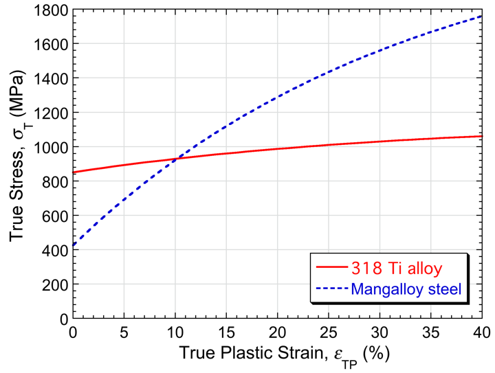
Figure 2. Stress-strain curves for the 318 Ti and Mangalloy alloys.
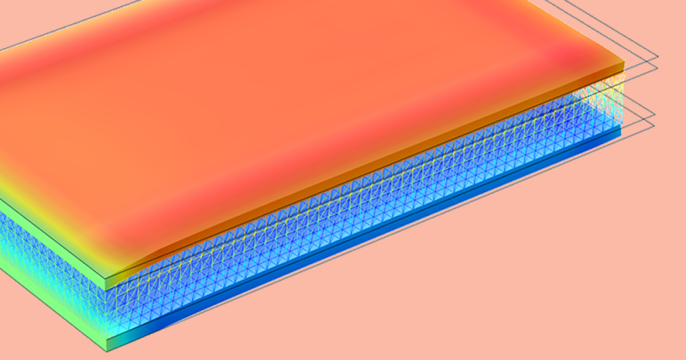
Fig. 3 shows predicted stress fields for Brinell and Vickers indent simulations that were conducted using COMSOL Multiphysics for the 318 Ti alloy. Figs. 4 and 5 present the corresponding outcomes of these simulations, in terms of residual indent profiles, for Brinell and Vickers tests carried out on these two alloys. In order to convert these profiles to hardness numbers, a judgment has to be made about what would be perceived as the diameter of the indent if it were to be viewed in the optical microscope. There is an element of subjectivity in this — or at least a dependence on imaging conditions — but the expected values are indicated in these figures, together with an estimated error range.
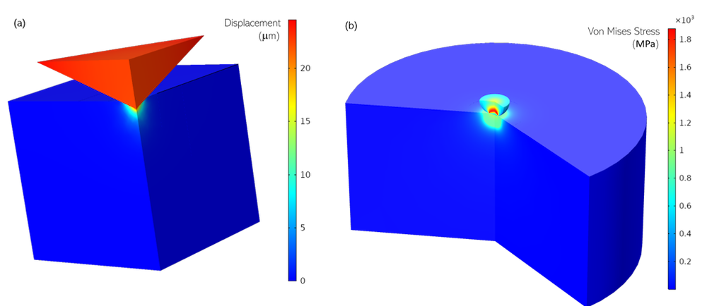
Figure 3. Predicted displacement field at the peak applied load of 5 kgf during a simulated indentation test with a Vickers indenter (left) and a predicted von Mises stress field during indentation with a Brinell indenter at a peak applied load of 3000 kgf (right).
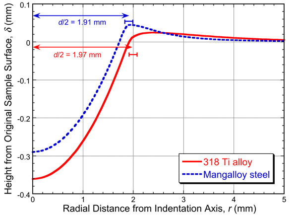
Figure 4. Predicted residual indent profiles for 318 and Mangalloy alloys after Brinell indentation.


Figure 5. Predicted residual indent profiles (across the long diameter) for 318 Ti (left) and Mangalloy (right) alloys after Vickers indentation, using 4 different loads.
The Brinell and Vickers hardness numbers obtained in this way are shown in Fig. 6. The indicated ranges correspond to the ranges in measured diameter shown in Figs. 4 and 5. Several points are immediately clear. One is that, despite the stress-strain curves for these two alloys being so different (Fig. 2), the hardness numbers that are obtained for them are similar — certainly within the kind of experimental error that is expected on the basis of how they are measured. It can also be seen that these error ranges are relatively large, particularly for the smaller (lower load) Vickers indents. Such variations are familiar to anyone who regularly makes such measurements. Furthermore, attempts to convert these hardness values to a well-defined parameter, such as the yield stress (using correlations such as those of Eqn. (3)), are also subject to very large errors. For both of these alloys, a value of around 800 MPa would be obtained, which is OK for the Ti alloy (because it work hardens so little), but is way off for the Mangalloy. While most people who obtain and use hardness numbers are familiar with the idea that they should be treated with care, in reality, the situation is somewhat worse than this: treating them as quantitative in any sense can be very misleading.
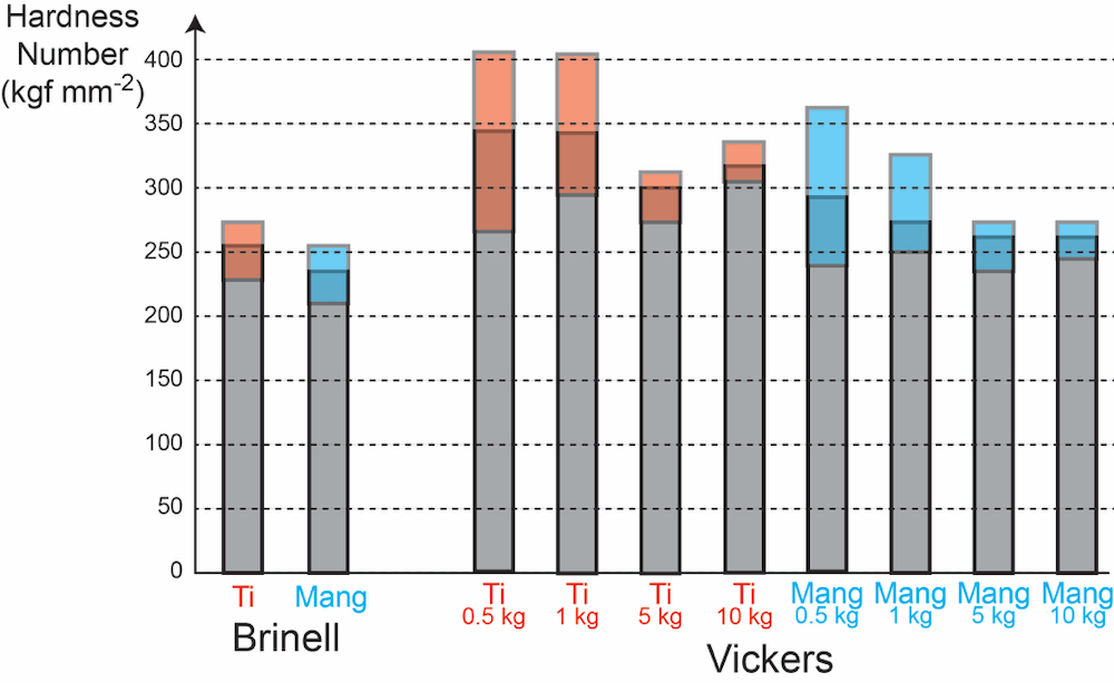
Figure 6. Hardness values derived from the indent diameter data shown in Figs. 3 and 4.
Indentation Plastometry
A potentially more useful test is one that incorporates the very best attributes of hardness testing (speed, simplicity, versatility) with the very best attributes of conventional tensile testing (namely the production of a full stress-strain curve). One such test method is Indentation Plastometry, which has been developed by scientists from Plastometrex. It involves three very simple steps:
- A spherical indent is created in the material (much like in the Brinell hardness test)
- The residual profile shape is measured using an integrated profilometer
- The residual profile data are analyzed in a bespoke software package that was developed using the Application Builder in COMSOL Multiphysics
The premise of the underlying method is conceptually very simple, involving repeated running of indentation finite element simulations (using COMSOL Multiphysics) until experimental datasets (residual profile shapes) and model predictions converge (after systematic alteration of the parameters in a constitutive plasticity law). However, there are several complicating factors, including issues of solution “uniqueness” and the identification of optimal test conditions. It is also clear that any such package (to be commercially viable) should provide the answers very quickly, so the convergence procedures need to be rapid and robust. The ones implemented by Plastometrex do in fact ensure that full stress-strain curves are obtained within a few seconds of the residual profile data being supplied. The whole test procedure, including creation of the indent and measurement of the profile, takes just three minutes.
SEMPID and the Application Builder in COMSOL Multiphysics®
A major attraction of the Application Builder is that it enables its users to create standalone applications that have access to the full power of COMSOL Multiphysics, with a licensing arrangement that permits the commercialization of such tools. Our own application, which implements the framework underpinning Indentation Plastometry, is called Software for the Extraction of Materials Properties from Indentation Data (SEMPID). The Application Builder was central to the development of SEMPID, thanks mainly to its wide range of native developer tools and its tight integration with COMSOL Multiphysics. The SEMPID application is able to leverage a number of core features of COMSOL Multiphysics, including the Structural Mechanics and Nonlinear Structural Materials modules, its suite of optimization tools, and its advanced solver setup features, to create a bespoke application, which now forms the basis of an entirely new company that boasts Element Materials Technology as its main investor.
Features of the SEMPID Software Package
The SEMPID application calculates stress-strain curves in both true and nominal form. There is, however, an additional feature, which allows users to simulate a tensile test in real time and enables the post-necking part of the stress-strain curve to be captured. The purpose of providing such a facility is to enable direct comparisons between stress-strain curves obtained by Indentation Plastometry and those obtained by conventional uniaxial tensile testing (which is, of course, the ultimate test of the validity of this new method).
Several screenshots of the SEMPID application are shown in Fig. 7, along with an image of an Indentation Plastometer. On display are a set of calculated stress-strain curves, along with results from tensile test simulations that were run from within the SEMPID application.

Figure 7. An Indentation Plastometer from Plastometrex and screenshots from the SEMPID software tool developed using the COMSOL Application Builder.
The Indentation Plastometer
The SEMPID software package comes bundled with the purchase of an Indentation Plastometer, which is a custom-built machine that fully automates the necessary test procedures, using programmed test protocols that adhere to confidential test routines developed in-house. The machine can handle a range of sample sizes and geometries, and it can accommodate real components that have parallel sides. It has fully integrated electronics, a maximum load capacity of 7.5 kN, an integrated profilometer, and custom-written control software. It is lightweight (<40 kg) and compact, allowing it to sit on a typical benchtop. A validation example is shown in Fig. 8 for a test conducted on Inconel 718, but the methodology is applicable to all metal types.

Figure 8. Shown on the left is the indent created by the Indentation Plastometer in a specimen of Inconel 718. To the right is a comparison between the SEMPID-derived stress-strain curve, and the stress-strain curve measured experimentally using a conventional mechanical test machine.
See the Indentation Plastometer in action in this quick video.
Reference
- S.K. Kang, J.Y. Kim, C.P. Park, H.U. Kim, and D. Kwon, “Conventional Vickers and True Instrumented Indentation Hardness Determined by Instrumented Indentation Tests”, Journal of Materials Research, 25(2): pp. 337–343, 2010.
About the Author
Dr. James Dean has an undergraduate degree in materials science from Imperial College, London, and a master’s degree in thermal power (gas turbine engineering) from Cranfield University, where he was supported with a Rolls Royce UTC Scholarship. He obtained his PhD from the Department of Materials Science at Cambridge University. He has since held research assistant and senior research associate positions in the same department, and in 2018, he joined the Centre for Scientific Computing at the Cavendish Laboratory as a senior teaching associate and coordinator of the Centre for Doctoral Training in Computational Methods for Materials Science. In 2012, he founded Double Precision Consultancy (DPC), which is a company based in Cambridge, UK, that specializes in the provision of advanced mathematical modeling services to industrial clients. DPC is now one of only five UK-based COMSOL Certified Consultants. In late 2018, he cofounded Plastometrex and is now its chief executive.


Comments (0)