The beauty of COMSOL is that it provides a unified modeling platform no matter what type of simulations you are performing. This is almost unique to the CAE market. Recently we showed you how to model chemical reactions using a monolith reactor as our example. First we walked you through solving the reaction kinetics and then involving plug flow, next we created a full-scale 3D model of the reactor. A chemical engineer may feel comfortable using a software optimized for this type of simulation, but what if he or she has to contemplate other properties in the device or process as well? For example, a catalytic converter is an exothermic reactor that sits near the exhaust of a car or truck, and there may be requirements for how long it must survive and function adequately before being replaced. In this final part of our “Modeling Chemical Reactions” blog series we will perform a thermal stress analysis of our converter.
3D Model of a Monolith Reactor Confirms Suggested Chemical Ratio
To recap what we did in the previous two blog posts, our reaction kinetics analysis and plug flow model suggested an NH3:NO ratio of 1.3, and our full 3D model of the monolith reactor confirmed this ratio. The 3D model also allowed us to understand how the system will work full-scale, leading us to one final analysis to carry out: thermal stress.

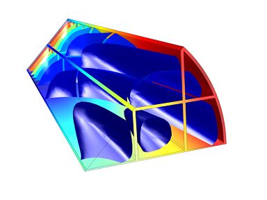
Model of selective NO reduction in a monolith reactor.
Performing a Thermal Stress Analysis
We’ve already determined what ammonia dosage we need for our system and what the reactor should look like. As we noted before, the monolith reactor experiences continuous change in temperature. Heat is generated by the chemicals, which dissipates into the surroundings at varying degrees throughout the system. This temperature flux along with the different material properties the structure is made up of can lead to thermal stress. Therefore, in order to truly optimize the reactor’s performance we need to analyze the thermal stress.
Let’s assume we have the 3D model we created in Part 2 of this series open in the Chemical Reaction Engineering Module. Before we can run our thermal stress analysis on the model, we need to extend it by coupling the temperature field to a structural mechanics analysis. The features and equations required for the stress analysis and general linear- and nonlinear solid mechanics are contained within the Solid Mechanics interface in the Structural Mechanics Module. These equations are the key to analyzing thermal expansion.
Thermal loads:
σ = Dεel + σ0 = D(ε–εth – ε0) + σ0
In this equation, σ is the stress, D is the elasticity matrix, and ε represents the strain.
Thermal strain:
εth = α(T – Tref)
Here α is the coefficient of thermal expansion, T is temperature (Kelvin), and Tref is the strain-free reference temperature (also Kelvin).
Results
Once we have solved for the physics and set up our model, it will look like this:

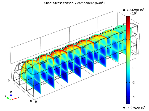
Stress tensor slice plot.
In the figure above you can see the stress tensor’s x-component plotted in several cross-sections. The deep blue color you see in the channel blocks, almost half-way up the channel, indicate high negative values, or compressive stresses. This is also where the tensile stresses (red color) are greatest. The region of greatest potential failure is therefore consistent with the temperature field shown in our 3D model.
On the other hand, we have the outer regions of our channels, in particular towards the end of the converter. Here, not many reactions were occurring: the temperature was lower and there were far less stresses. In short, we can evaluate our maximum compressive stress to be about 5.0 MPa and tensile stress around 7.2 MPa. (During system start-up stress levels are expected to be more significant).
Conclusion and Next Steps
With this thermal stress analysis we have now concluded our “Modeling Chemical Reactions” blog series. We have gone through analyzing the kinetics, created a plug flow model, developed a full-scale model, and even investigated other physics that affect the system’s performance. Now we know what ammonia dosage is necessary, what the system will look like, and how it will perform. Next steps are up to you — perhaps you can try modeling this multiphysics problem on your own?


Comments (0)