

One of the perennial questions in finite element modeling is how to choose a mesh. We want a fine enough mesh to give accurate answers, but not too fine, as that would lead to an impractical solution time. As we’ve discussed previously, adaptive mesh refinement lets the software improve the mesh, and by default it will minimize the overall error in the model. However, we often are only interested in accurate results over some subset of the entire model space. Today we will introduce a technique to refine the mesh based on a local metric.
A Model with Global Mesh Refinement
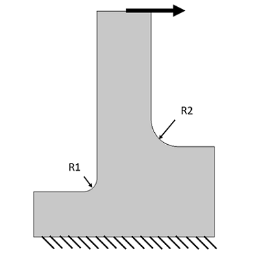
Let’s take a look at a simple mechanical problem — a bracket that is fixed at the bottom and has a load applied at the top. Two different fillet radii are applied and, as a consequence, it is difficult to predict where the peak stresses will be. Let’s first solve the problem on an extremely coarse mesh, using the default second-order elements, and observe the results. We can see that the peak stresses are at the larger radius fillet, and that the mesh appears to quite poorly resolve the solution.

Stresses and deformations solved on a coarse mesh.
To get a more accurate solution, we can go to the Adaptation and Error Estimates settings available with the Stationary, Frequency Domain, and Eigenvalue study steps. An example of these settings is shown in the screenshot below. The error estimate is by default based upon minimizing the L2 norm of error squared, which is a global metric. That is, the remeshing will reduce the error everywhere in the model. The default refinement method is Mesh initialization, which will refine the mesh in areas where smaller elements are needed, but can also coarsen the mesh where a fine mesh is not needed. By default, this adaptive refinement will be done twice, but in the screenshot below, a total of four refinements are specified.
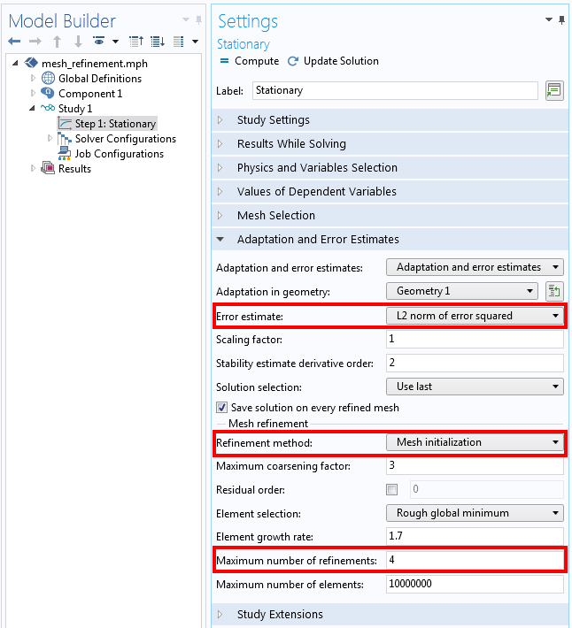
Adaptive mesh refinement settings to reduce the global error in the model. Relevant settings are highlighted.
The result of this adaptive mesh refinement is shown below. Note how the mesh is quite uniformly refined throughout the domain. The stress field is clearly smoother than on our original mesh.
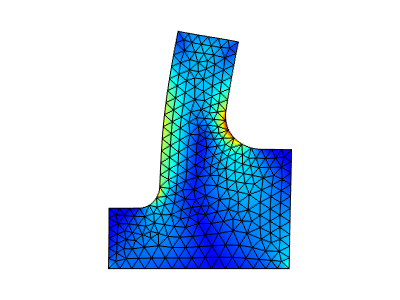
The results of the adaptive mesh refinement using the L2 norm of error squared as the error estimate.
Local Solution-Based Adaptive Mesh Refinement
Let’s now set up the same problem, but use a different metric for the adaptive mesh refinement. From the coarse mesh, we can probably already see that the highest stresses are at the larger radius fillet so we can tell the adaptive mesh refinement algorithm to address the stresses in this location. We will switch to a Functional Error Estimate, which requires that we enter a functional with respect to which the mesh will be improved. The functional can be any differentiable scalar output based upon the solution. The functional we will use is the integral, along the boundary, of the von Mises stress, the model variable comp1.solid.mises. An Integration component coupling named comp1.intop1() is defined at the boundary defining the larger fillet, as shown in the screenshot below.
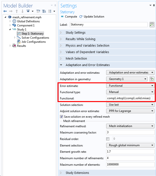
Adaptive mesh refinement settings to reduce the local error at one location in the model.
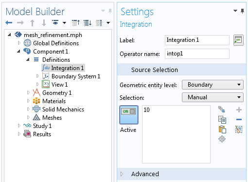
The Integration coupling operator is used to define the boundary where we will evaluate the stress.
When we look at the results of this approach, we should notice two features of the refined mesh. First, it has preferentially inserted smaller elements around the fillet boundary that we selected. This is as expected, since we are trying to get more accurate results in this region. However, we also observe that the mesh has been refined in other regions of the model, not just at the boundary of interest. The adaptive mesh refinement algorithm will globally adjust the mesh to better resolve the local stresses, and these stresses depend on the solution everywhere else in the model.
We can also see that using manual mesh refinement to predict the peak stress may be very difficult, because we usually cannot easily determine what other parts of the model may affect our solution.

The refined mesh, based upon a local functional error estimate.
Conclusions on Adaptive Meshing
We have seen that you can specify a local quantity over which to perform adaptive mesh refinement, and the software will refine the mesh to give better results locally, but also refine the mesh in other regions of the model that you may not immediately realize affect the local quantity you are interested in. The technique shown here is a powerful way to refine the mesh with confidence.
Editor’s note: This blog post was updated on 8/21/17.


Comments (19)
Marvin Farrell
August 25, 2014Here I am wondering how to set the parameters to get the accurate results? Thanks
Walter Frei
August 25, 2014Thank you Marvin, When reading this article, keep it in the larger context of solving multiphysics problems:
http://www.comsol.com/blogs/learning-solve-multiphysics-problems-effectively/
In particular, meshing considerations are a topic we’ve addressed before:
http://www.comsol.com/blogs/how-to-implement-mesh-refinement-study/
http://www.comsol.com/blogs/meshing-considerations-linear-static-problems/
Roberto Gaddi
December 21, 2015I have a question about the functional: does it need to be a function that converges to zero as the mesh quality improves? Does the adaptive mesh algorithm try to minimize this quantity? Or is the error calculated as the delta of the functional in between steps, so the algorithm is looking for a stable value of the functional? In my case the functional is a quantity that would converge to a non-zero value. Is this going to work?
A second question is about the use of “Longest” vs. “Mesh Initialization” as refinement method: I cannot find an explanation on what the difference is an I cannot chose the best for my model.
Thanks,
Roberto
Walter Frei
December 21, 2015Hello Roberto,
The functional you choose does not need to converge to zero, no. In the case shown here, for example, it does not converge to zero. The algorithm is improving the accuracy of this functional by adjusting the mesh.
Regarding “Longest” vs. “Mesh Initialization”. The “longest” or “regular” methods will always work, but will only refine the mesh. The “mesh initialization” can both refine and coarsen the mesh but may, in rare circumstances, fail. There is no one method which will always be best for every case, you may want to try both.
Chinmoy Mallick
March 1, 2016Hi,
I’m doing simulations to find a contour or surface having 875 gauss field.I’ve two permanent ring magnets and i want to visualize the 2D field.while doing adaptive mesh confine following error coming during simulations……Pl can anyone tell me where is the error?..Thank you
“Failed to find a solution.
Attempt to evaluate negative power of zero.
Function: ^
Failed to evaluate temporary symbolic derivative variable.
Variable: comp1.mf.normBVDN${realdot7}, Defined as: (((realdot(comp1.mf.Br,comp1.mf.Br)+realdot(comp1.mf.Bz,comp1.mf.Bz))^(-0.5))*0.5)
Failed to evaluate expression.
Expression: d((comp1.mf.normB-0.087499999999999994),{realdot7})
Returned solution is not converged.
– Feature: Stationary Solver 1 (sol3/s1)”
Bridget Cunningham
March 1, 2016Hello Chinmoy,
Thank you for your comment.
For questions specific to your modeling work, please contact our support team.
Online support center: https://www.comsol.com/support
Email: support@comsol.com
Soma Sai Sriram Kumar Bysani
April 7, 2017Hello,
My geometry is 3D I am designing a heat exchanger and similations are done in comsol 5.2a multiphysics. In my geometry one is heat domain and other one is fluid domain. The velocity profile in the fluid domain was not accurate, I want increase elements of fluid domain only can someone please help how to proceed it?
Now total elments in fluid domain are 280,000K
I need in that domain like 550,000K
Caty Fairclough
May 3, 2017Hi,
Thanks for your comment!
For questions related to your modeling, please contact our Support team.
Online Support Center: https://www.comsol.com/support
Email: support@comsol.com
Joerg Ruediger
August 3, 2017Hi Walter,
I cannot find the Adaptive Mesh Refinement – node under stationary solver. How to enable it?
Joerg
Caty Fairclough
August 4, 2017Hi Joerg,
Thank you for your question.
I would suggest contacting our Support team for questions related to your modeling.
Online Support Center: https://www.comsol.com/support
Email: support@comsol.com
Kelvin Leung
March 20, 2018Hi Walter,
Is adaptive meshing available for time dependent solution?
Kelvin
Walter Frei
March 29, 2018Yes, adaptive mesh refinement is available for time-domain models. See, for example:
https://www.comsol.com/model/inkjet-1445
Dheeraj Kumar
May 28, 2018Thanks Walter
Do you also have the associated model files?
Regards
Dheeraj
Walter Frei
May 29, 2018Hello Dheeraj,
The user interface has changed a bit since this blog was written. We do have updated examples showing the usage of adaptive mesh refinement, for example:
https://www.comsol.com/models/?q=%22adaptive+mesh%22
In particular, the simplest is:
https://www.comsol.com/model/implementing-a-point-source-73
Best Regards,
Mohammadreza Mohaghegh
May 12, 2021Hello Walter,
First of all, thank you for your helpful comments, prompt replying, and your time, really appreciated.
I am using COMSOL 4.3b, and gonna use adaptive mesh refinement for a melting PCM problem (time-dependent) to use enough fine mesh in the phase change interface zoon (melting front). What should I need to do so? just checking the box of daptive mesh refinement in the study module? any other control parameters or? How this model can detect the transition zone (melting front)? (I have an input, dT1 as a thickness of transition layer)
Thanks
Muzammil Nawaz
August 6, 2019Hello,
I cannot see ” Adaption and Error Estimate ” Node in Settings window of Stationary study. I am using COMSOL 5.2. Please help me in this regard.
Thanking in anticipation.
Ivar KJELBERG
March 30, 2020Hello Walter
This blog requires some updates following your now important changes in the V5.5 “Adaptation and Error Estimates” section that has been “improved”, hopefully, but neither the help/documentation nor this blog is very useful anymore as none seem to define nor follow your new terminology …
Sincerely
Ivar
Chengzhe Zou
May 18, 2020Hi Walter, great post! I have a question on error estimation. When you talk about error, this implies that you know the exact value. But before mesh refinement, the coarse mesh cannot give you the exact value. So how does COMSOL estimate the error? Thank you!
Walter Frei
May 12, 2021 COMSOL EmployeeHello Chengzhe,
It is not quite the case that this article on error was meant to imply that the exact value is known, no. (Except in some analytic cases, of course…) The question of error estimation for adaptive mesh refinement (emphasis on *estimation*!) is a non-trivial subject.
There is a section in the Reference Manual, titled “Error Estimation — Theory and Variables” that provides more details as well as references for further reading.