La Bibliothèque d'Applications présente des modèles construits avec COMSOL Multiphysics pour la simulation d'une grande variété d'applications, dans les domaines de l'électromagnétisme, de la mécanique des solides, de la mécanique des fluides et de la chimie. Vous pouvez télécharger ces modèles résolus avec leur documentation détaillée, comprenant les instructions de construction pas-à-pas, et vous en servir comme point de départ de votre travail de simulation. Utilisez l'outil de recherche rapide pour trouver les modèles et applications correspondant à votre domaine d'intérêt. Notez que de nombreux exemples présentés ici sont également accessibles via la Bibliothèques d'Applications intégrée au logiciel COMSOL Multiphysics® et disponible à partir du menu Fichier.

Ray Release Based on a Plane Electromagnetic Wave
This tutorial shows how to set up a ray release based on the incident electric field at a boundary. First the Electomagnetic Waves, Frequency Domain interface is used to solve for the electric field of a plane wave. Then rays are released with initial intensity and polarization matching ... En savoir plus
Component Mode Synthesis Tutorial
In this tutorial example, the concepts of Component Mode Synthesis (CMS) are introduced through a simple solid model of a cantilever beam. Parts of the beam are reduced by the CMS technique. It is, furthermore, shown how CMS can be used to represent both the static and dynamic behavior ... En savoir plus
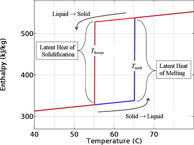
Modeling Phase Change with Hysteresis
This example exemplifies how to model thermal phase change that is subject to hysteresis. A more detailed description of the phenomenon, and the modeling process, can be seen in the blog post "Thermal Modeling of Phase-Change Materials with Hysteresis" as well as: "How to Use State ... En savoir plus

Compact Camera Module
Compact camera modules are widely used in electronic devices such as mobile phones and tablet computers. In order to reduce both the size and number of elements required the optical design will typically incorporate several highly aspheric surfaces. This model demonstrates a five element ... En savoir plus
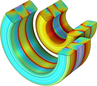
Electromagnetic Force Calculation Using Virtual Work and Maxwell Stress Tensor
The model compare the electromagnetic force calculated by virtual work and maxwell stress tensor methods on the axial magnetic bearing. The forces is evaluated by studying the effect of a small displacement on the electromagnetic energy of the system. This is done by using the Magnetic ... En savoir plus

Coil Optimization of an ICP Reactor
This model shows how shape optimization can be used design the coils of an ICP reactor to obtain plasma uniformity. The reactor in study is a planar ICP with the coils distributed along the radial direction. The Optimization study step is used to find the best coil placement so that the ... En savoir plus
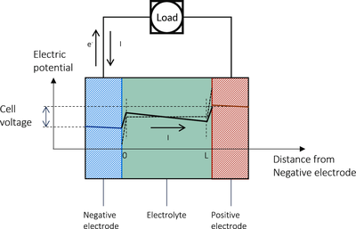
Potential Profile in Batteries and Electrochemical Cells
The purpose of this model is to visualize the electric potential in an electrochemical cell, for example a battery. This is done at OCV and during operation. In a battery, this would correspond to OCV, discharge, and recharge. The potential profile is explained both for cells with planar ... En savoir plus

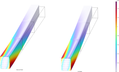
Convective Heat Transfer with Pseudo-Periodicity
This model simulates convective heat transfer in a channel filled with water. To reduce memory requirements, the model is solved repeatedly on a pseudo-periodic section of the channel. Each solution corresponds to a different section, and before each solution step the temperature at the ... En savoir plus

Polynomial Hyperelastic Model
This model shows how you can implement a user defined hyperelastic material, using the strain density energy function. The model used is a general Mooney–Rivlin hyperelastic material model defined by a polynomial. In this example, you will see two material models based on the defined ... En savoir plus

Generating a Simulation Mesh From Scanned Data
See how to generate a mesh from scanned data via two different workflows. For both examples, the data file is imported in an Interpolation function. In the first workflow, the data is applied on a Grid dataset and a Filter dataset is used to filter out the data to represent the femur. ... En savoir plus