

This past July, I had the pleasure of attending the 22nd International Congress on Sound and Vibration. In addition to running the COMSOL vendor booth with my Italian colleague Gabriele, I was also a presenter at the event. My presentation was based on a paper I wrote with Henrik Bruus and Jonas Karlsen that focuses on how to determine acoustic radiation forces including thermoviscous effects. Let’s explore acoustophoretic effects in greater detail and the research findings highlighted in my presentation.
What Is Acoustic Radiation Force?
Acoustic radiation force arises due to momentum transfer from an acoustic field to a small particle, which results in a net force acting on the particle. In the related phenomenon of acoustic streaming, a net fluid flow is driven by an acoustic field, with momentum transfer (to the fluid) occurring in the acoustic boundary layer.
Both phenomena are important as they are used to move, control, and sort particles or small living organisms (i.e., cells, proteins, or large viruses) in, for instance, microfluidic devices. This kind of particle manipulation is known as acoustophoresis, that is, movement by sound. The radiation force acts directly on the particle while acoustic streaming induces drag on the particles. The magnitude and/or direction of the effects depends on the size and mechanical properties of the particles as well as the fluid properties. A solid understanding of such phenomena is essential for producing and optimizing devices to efficiently sort and manipulate particles. In a previous blog post, I demonstrated how to model the acoustic radiation force and acoustic streaming in a microfluidic device.
My presentation at the 22nd International Congress on Sound and Vibration (ICSV22) was an extension and generalization of how to model the acoustic radiation force in detail using the so-called second-order perturbation theory. The Acoustophorectic Force blog series provides a helpful introduction to understanding the radiation forces as well as different ways to compute these forces.
Different Approaches to Analyzing Acoustic Radiation Forces
Let’s now get a bit more technical and pull out a few equations. As is the case for most physics problems, there are several ways of describing and deriving the radiation force effect under different physical assumptions and in different regimes. I will briefly summarize and describe these different approaches here.
Direct FSI Approach
In the direct fluid-structure interaction (FSI) approach, the full (nonlinear) set of governing equations is solved as a dynamic problem. The radiation force is then extracted by looking at the time-averaged particle motion. In order to include both thermal and viscous losses, the Navier-Stokes equations need to be solved together with the energy equation, which is, in essence, nonisothermal flow. The equations should be solved with high numerical precision in order to capture all of the small-scale effects associated with the radiation force.
Second-Order Perturbation Approach
To simplify the analysis of the full set of nonlinear governing equations, the problem can be split up into a linear acoustic problem and a linear time-averaged second-order problem. This is accomplished via the second-order perturbation theory; for example, the pressure p is written as p = p_0+p_1+p_2. Subscript 0 represents background properties (the 0th pressure could be roughly a constant single atmosphere, depending on equilibrium conditions), subscript 1 represents the classical acoustic fields, and subscript 2 represents the second-order perturbation fields needed to capture the nonlinear effects. The different-order equations are solved sequentially.
This theory establishes that, in general, the radiation force on an object \Omega is given by
(1)
where \langle \cdot \rangle represents time averaging, \sigma_2 is the second-order contribution to the stress, \mathbf{u}_1 is the acoustic variation in the velocity field, and the integral is on any closed surface surrounding the particle.
Thus, in order to find the radiation force, the acoustic problem (first-order perturbation) and the second-order perturbation equations must both be solved. This method was used in the research presented at ICSV22, which we will discuss in greater detail below. The equations are solved, including thermal and viscous losses in both fluids and solids.
The No Loss Limit
The fluid can be treated as having no loss for particles of size a much larger than the viscous and thermal boundary layers (the penetration depth \delta_\textrm{tv}), that is, \delta_\textrm{tv}/a \ll 1. In this case, the second order-stress in Eq. (1) can, in the far-field, be simplified to
(2)
By determining the scattered field p_1 and \mathbf{u}_1 of any object, the radiation force in Eq. (1) can be calculated. It is not necessary to know the second-order fields explicitly. Ref. 2 in our Further Reading section and the blog post “How to Compute the Acoustic Radiation Force” provide two examples of this.
The Rayleigh Limit
In the Rayleigh limit, the particle is assumed to be acoustically small. That is, k\cdot a \ll 1, where a is the particle size and k is the wave number. Scattering theory is used to derive the scattered field off the particle. In this limit, the radiation force given in Eq. (1) reduces to
(3)
where f_0 and f_1 are the monopole and dipole scattering coefficients and the subscript \textrm{in} represents the incident acoustic field (e.g., the standing acoustic field in a sorting device) evaluated at the small particle’s location. The fluid compressibility is \kappa_s and the fluid density is \rho_0.
The whole gymnastics of this approach consists within finding the two scattering coefficients. Several analytical results exist:
- In the inviscid and adiabatic case, the results are given by Gor’kov in Ref. 3.
- Results including viscosity are given by Settnes and Bruus in Ref. 4.
- In Ref. 5, a full thermoviscous theory is given by Karlsen and Bruus. Here, the scattering is also solved off a small droplet, and the thermoviscous effects are included inside the particle as well.
- Many results in this field can be found in so-called suspension acoustics (see Ref. 6).
Equation-Based Modeling in COMSOL Multiphysics
As a first model system, we decided to determine the acoustic radiation force acting on a small spherical particle placed in an ultrasonic standing wave. As mentioned above, we opted to use the detailed perturbation approach to find the radiation force, as given in Eq. (1). The model included thermal and viscous losses in fluids and solids.
The first step was to determine the acoustic fields (the first-order field); in other words, solve the equations in the Thermoacoustics, Frequency Domain physics interface in fluids, coupled to the Thermoelasticity interface in solids. The coupling required is not predefined in COMSOL Multiphysics, but it can easily be set up in the user interface (UI). COMSOL Multiphysics will then solve the problem fully coupled.
Once the first-order fields have been established, the equations for time averages of the second-order equations can be solved. So, from here on we shall omit the \langle \cdot \rangle notation for the second-order quantities and whenever they appear in the equation, they will be understood in their time-averaged sense, \langle a_2 \rangle \equiv a_2.
The structure of these equations is identical to the laminar flow equations in the CFD Module, with the addition of source terms. For numerical reasons, we chose not to use the predefined equations, but rather implement our own version cast into the conservative form. This step is important for reducing the numerical noise propagating from the first-order field to the second-order solution. In the nonconservative formulation, gradients of the first-order fields need to be evaluated explicitly, thus introducing numerical noise. The equations for mass, momentum, and energy conservation are:
(4)
\nabla\cdot[\rho_0 \mathbf{u}_2+\langle \rho_1 \mathbf{u}_1 \rangle] = 0 \\
\nabla\cdot [\mathbf{\sigma}_2 – \rho_0\langle\mathbf{u}_1\mathbf{u}_1^\textrm{T}\rangle \mathbf] = \mathbf{0} \\
\nabla\cdot [k \nabla T_2+\langle \mathbf{u}_1\cdot\mathbf{\sigma}_1\rangle + \alpha_0 T_0 \langle p_1 \mathbf{u}_1 \rangle – \rho_0 C_\textrm{p}\langle T_1 \mathbf{u}_1 \rangle] = 0
\end{aligned}
where it is assumed that the second-order fields are time-averaged values. Notice that the first-order fields play the role of source terms in the second-order equations.
Setting up the equations and boundary conditions was only possible using the general weak form available in COMSOL Multiphysics. The flexibility to add and define new equations was paramount to solving this problem.
The Results
We’ve covered the theory and equations. Now we can move on to looking at some nice, colorful results.
As a system example, let’s have a look at a small spherical polystyrene particle of radius from a=1 \: \mu \textrm{m} to a=40 \: \mu \textrm{m}. The particle is surrounded by air and is located in a standing 2 MHz ultrasound field, which gives \delta_\textrm{v} = 1.6 \: \mu\textrm{m} and \delta_\textrm{t} = 1.9 \: \mu\textrm{m}. Thus, for the smaller particles, boundary layer effects are expected to be significant and the lossless theory inaccurate. Moreover, for the large particles, we are outside the Rayleigh limit, k\cdot a \ll 1, with 0.04 < k\cdot a < 1.5 for the chosen particle-size range. This means that we are outside the range of the analytical theories.
The oscillating acoustic pressure field.
The animation above depicts the total harmonically oscillating acoustic pressure field p_1. The black circles represent different integration surfaces used to evaluate Eq. (1), but they are also used to control the computational mesh. The scattered field off the particle is illustrated below. This harmonic pressure oscillation leads to a net time-averaged radiation force because of nonlinear effects.
The scattered field off the particle.
The series of animations below illustrate results from a range of simulation analyses. In the top row, the figure on the left depicts temperature fluctuations T_1 around the particle. The extent of the temperature variations indicates the thermal boundary layer or penetration depth into the fluid. The figure on the right shows the deformation of the small polystyrene particle as well as the first-order temperature variations in the solid. Here, the thermal penetration depth inside the solid is again captured. Moving down to the bottom row, the figure on the left represents the axial velocity component of the scattered acoustic field, while the figure on the right indicates the radial velocity component of this field.
Results from a range of simulation analyses. Top left: Temperature variations. Top right: Deformation of the particle. Bottom left: Axial velocity component of the scattered acoustic field. Bottom right: Radial velocity component.
We can plug the first-order fields into the second-order equations — see Eq. (4) — and then solve for a local steady-state streaming flow around the particle. The pressure and velocity magnitude are shown in the next two figures, respectively. Take note of the very small scale (indicated by the color bars) for the pressure (unit: Pa) and the velocity (unit: m/s). Take, for example, the pressure relative to the incident driving wave, which has an amplitude of 3\cdot 10^{-3} \: \textrm{Pa}.
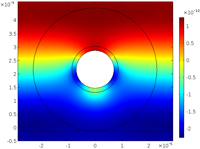
Pressure field.
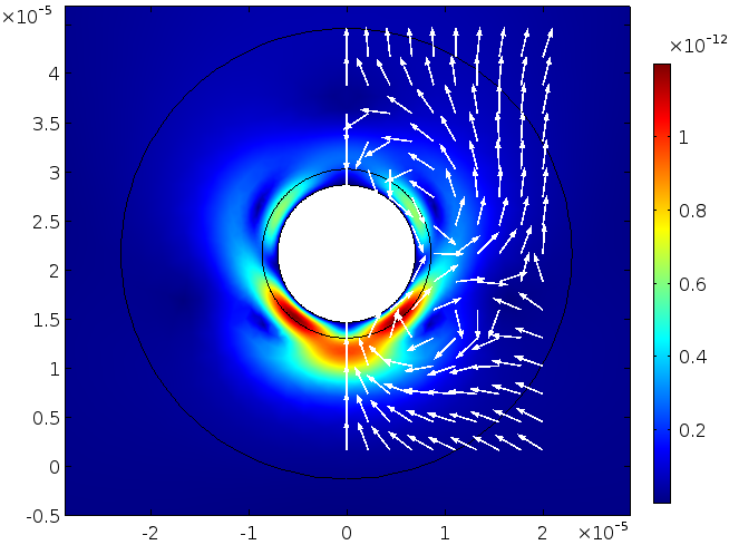
Velocity field.
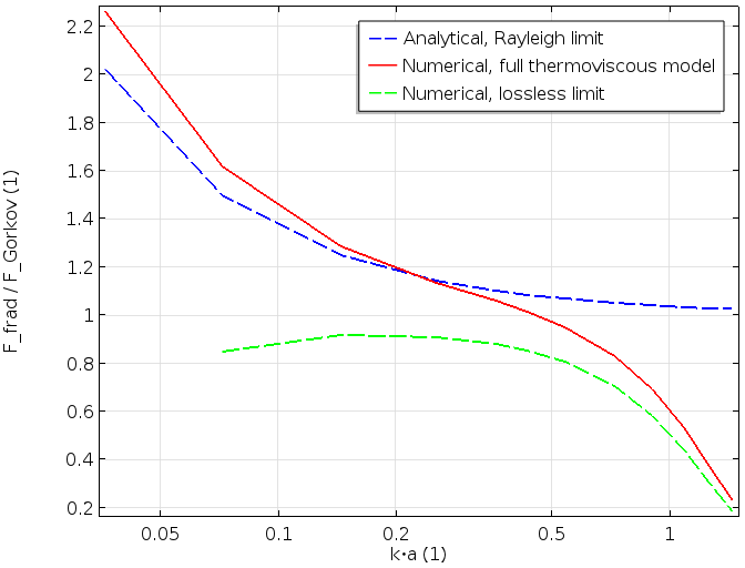
Finally, once the first-order and second-order fields are known, we can derive the force given in (1). In the first graph, the force is depicted as a function of \delta_\textrm{v}/a (viscous penetration depth over particle size). In the second graph, it is depicted as a function of k\cdot a. The radiation force is nondimensionalized by the corresponding force evaluated in the lossless case and in the Rayleigh limit (denoted by Gor’kov).
These graphs include three curves. The blue dashed curve is the analytical expression given by Karlsen and Bruus in the Rayleigh limit. The green dashed curve indicates the force evaluated with the lossless model (disregarding the boundary layers) given in Eq. (2). Lastly, the red curve represents our full numerical model, including thermoviscous losses, which is valid for both large and small particles.
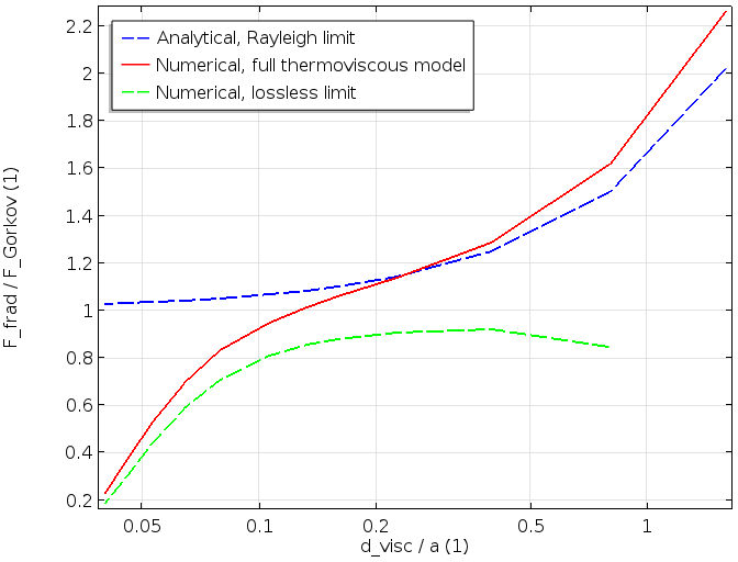
The first graph (shown above) illustrates how the full model with viscous and thermal losses connects the lossless (\delta_\textrm{v}/a small) to the blue curve, which includes losses but is only valid for small particles (large \delta_\textrm{v}/a for constant material parameters). The second graph, which is depicted below, shows the same characteristic. The detailed thermoviscous model that we implemented connects the large particle limit (green dashed curve lossless) and the small particle limit (blue dashed curve, small k\cdot a in the Rayleigh limit).
Concluding Remarks
Attending ICSV22 gave me the opportunity to present a small portion of the research that I have worked on with Henrik Bruus and his research group at the Technical University of Denmark. In parallel with experiments and numerical modeling, the research group’s work has facilitated a deep theoretical understanding of acoustophoretic phenomena.
My presentation focused on a new numerical full thermoviscous analysis of the radiation force acting on small spherical particles (ellipsoidal particles are planned for future studies). The model agrees well with existing results in their limit of applicability (the Rayleigh limit and/or lossless limit). As this method is very general, it can be readily extended to particles of an arbitrary shape. The model can also be further expanded to include more detailed material dependencies like the fluctuation of viscosity with temperature.
Further Reading
- “Theory and Simulation of the Acoustic Radiation Force on a Single Microparticle in an Ultrasonic Standing Wave Including Thermoviscous Effects”, M. J. H. Jensen, J. T. Karlsen, and H. Bruus.
- “Efficient finite element modeling of radiation forces on elastic particles of arbitrary size and geometry”, P. Glynne-Jones, P. P. Mishra, R. J. Boltryk, and M. Hill.
- “On the forces acting on a small particle in an acoustical field in an ideal fluid”, L. P. Gor’kov.
- “Forces acting on a small particle in an acoustical field in a viscous fluid”, M. Settnes and H. Bruus.
- “Forces acting on a small particle in an acoustical field in a thermoviscous fluid”, (accepted) J. T. Karlsen and H. Bruus.
- Suspension Acoustics: An Introduction to the Physics of Suspensions, S. Temkin.


Comments (13)
Ulrik Fallrø
January 19, 2018Hello Mads! Is there any possibilities to see guidelines for modeling the radiation force in COMSOL? I have a problem quite similar to the one in: https://www.comsol.com/blogs/how-to-compute-the-acoustic-radiation-force/. I am modelling the displacement on a microcalcification embedded in soft tissue when ultrasound is induced. The calc-particle is arbitrary large, so I have though to calculate as in “Second-Order Perturbation Approach”.
Jason Collins
September 18, 2020Hi Mads,
It would have been great if you had provided boundary conditions for implemented equations you used, I don’t understand what are the boundary conditions for sigma2.
Kind regards
Mads Herring Jensen
September 20, 2020 COMSOL EmployeeHi Jason,
Sigma 2 is the stress tensor in the laminar flow equations that describe the streaming flow around the particle. The equations in 4 are flow equations for the second order time averaged fields with source terms that stem from the first order acoustic fields. Note that you do not need to compute the streaming flow to compute a radiation force. We only did this for verification. If you compute the scattered acoustic field off the object, then use equation 1 and 2 (on a boundary surrounding the object, outside of the viscous layer) to compute the radiation force.
Best regards
Mads
Jason Collins
September 21, 2020I appreciate your prompt response, points you made really helped me understand equations. There is just one more thing that I’d be grateful if you tell me about so I have a deeper understanding of your model, your solid first interacts with p1 and u1 (thermoviscous) after this step solid particle interacts with laminar flow(p2 and u2) (fluid-structure interaction)?
Thanks
Jason
Mads Herring Jensen
September 21, 2020 COMSOL EmployeeHi Jason
If I remember correctly we just kept the particle fixed in the flow part. I think that is consistent with the second order perturbation approach.
Best regards
Mads
Jason Collins
September 24, 2020Hi Mads,
I tried my best to understand how you created your standing wave of 2MHz in thermoviscous, but I’m clueless so I desperately ask if you could tell me. I appreciate your responses so far.
I’m looking forward to hear more from you.
Kind regards
Jason
Mads Herring Jensen
September 24, 2020 COMSOL EmployeeHi Jason
First solve a model to determine a standing wave (no particle), then solve a second model where the standing wave field is used as a background acoustic field in a scattering problem. In the second problem use open conditions like a PML. I believe that in one of the referenced papers there is an analytical solution to a standing wave problem. So instead of solving for the standing wave you can use an analytical expression also. I might have used that expression, if I remember correctly.
Best regards
Mads
雅静 王
May 27, 2021Hi Mads,
Thank you very much for your article for providing me with very important ideas. Your results are also very beautiful and colorful, but how do you do the post-processing animation? Especially the vibration sound pressure field and the animation of particle deformation. Is this animation based on the time domain or the frequency domain?(or how to create the animation only in the research state of frequency?)
Best regards
Yajing
雅静 王
May 17, 2021Hi Mads,
Thank you very much for your article for providing me with very important ideas. Your results are also very beautiful and colorful, but how do you do the post-processing animation? Especially the vibration sound pressure field and the animation of particle deformation. Is this animation based on the time domain or the frequency domain?
Best regards
Yajing
Mads Herring Jensen
May 27, 2021 COMSOL EmployeeDear Yajing
The results are based on the frequency domain model. When you set up an animation (under the Export node) you can select what type of animation you want to perform. In this case it is a Dynamic Data Extension which automatically adds the phase “exp(i*omega*t)” to a frequency domain model, so that you can visualize it in time.
Best regards
Mads
雅静 王
May 30, 2021Dear Mads:
Thank you so much for your response and advice, which solved my recent problem. It is so great!
Best regards
Yajing
Andre Rieger
September 17, 2021Dear Mads,
I really hope to get an answer here, regarding the fact the article is quite old already
I was wondering whether or not the second order time average stress in eq. 1 and 2, respectively, is a tensor or just a scalar.
In both cases I have the problem of extract ing the direction of the force on the sxcatterer. Is the force direction completely determinded by the direction of the normal to the scatterers surface? Or is the second order Stress indeed a tensor? If so, what are the components? From the computation shown in eq. 2 it seems that all variables involved are scalar quanzities.
Sorry if my question seems simple. I am New to the topic and was wondering about this. Since I couldnt find an answer myself, I thought I just ask here.
Hope you can help.
Best reagrds,
André.
Mads Herring Jensen
October 1, 2021 COMSOL EmployeeHi André
The force in Eq 1 is a vector and what is dotted with the normal (under the integration) is a tensor. sigma2 is the stress tensor in the streaming flow. I believe there are variables for the magnitude of sigma.n available in the CFD interfaces in COMSOL. In Eq 2 in the lossless limit sigma2 reduces to the streaming pressure (so it is a diagonal tensor actually, p2 dot I), which is then approximated by the first order fields.
The direction comes from integrating the vector expression over the surface. In this case it ends up only having a contribution in the z-direction, due to symmetries.
Best regards
Mads