

Previously on the blog, we have discussed the need for appropriate measured data to fit the material parameters that correspond to a material model. We have also looked at typical experimental tests, considerations for operating conditions when choosing a material model, and an example of how to use your measured data directly in a nonlinear elastic model. Our focus today will be on how to fit your experimental data to different hyperelastic material models.
Curve Fitting in COMSOL Multiphysics
After obtaining our measured data, the question then becomes this: How can we estimate the material parameters required for defining the hyperelastic material models based on the measured data? One of the ways to do this in COMSOL Multiphysics is to fit a parameterized analytic function to the measured data using the Optimization Module.
In the section below, we will define analytical expressions for stress-strain relationships for two common tests — the uniaxial test and the equibiaxial test. These analytical expressions will then be fitted to the measured data to obtain material parameters.
Isotropic, Nearly Incompressible Hyperelasticity
Characterizing the volumetric deformation of hyperelastic materials to estimate material parameters can be a rather intricate process. Oftentimes, perfect incompressibility is assumed in order to estimate the parameters. This means that after estimating material parameters from curve fitting, you would have to use a reasonable value for bulk modulus of the nearly incompressible hyperelastic material, as this property is not calculated.
Here, we will fit the measured data to several perfectly incompressible hyperelastic material models. We will start by reviewing some of the basic concepts of the nearly incompressible formulation and then characterize the stress measures for the case of perfect incompressibility.
For nearly incompressible hyperelasticity, the total strain energy density is presented as
where W_{iso} is the isochoric strain energy density and W_{vol} is the volumetric strain energy density. The second Piola-Kirchhoff stress tensor is then given by
where p_{p} is the volumetric stress, J is the volume ratio, and C is the right Cauchy-Green tensor.
You can expand the second term from the above equation so that the second Piola-Kirchhoff stress tensor can be equivalently expressed as
where \bar{I}_{1} and \bar{I}_{2} are invariants of the isochoric right Cauchy-Green tensor \bar{C} = J^{-2/3}C.
The first Piola-Kirchhoff stress tensor, P, and the Cauchy stress tensor, \sigma, can be expressed as a function of the second Piola-Kirchhoff stress tensor as
\sigma& = J^{-1}FSF^{T}
\end{align}
Here, F is the deformation gradient.
Note: You can read more about the description of different stress measures in our previous blog entry “Why All These Stresses and Strains?“
The strain energy density and stresses are often expressed in terms of the stretch ratio \lambda. The stretch ratio is a measure of the magnitude of deformation. In a uniaxial tension experiment, the stretch ratio is defined as \lambda = L/L_0, where L is the deformed length of the specimen and L_0 is its original length. In a multiaxial stress state, you can calculate principal stretches \lambda_a\;(a = 1,2,3) in the principal referential directions \hat{\mathbf{N}_a}, which are the same as the directions of the principal stresses. The stress tensor components can be rewritten in the spectral form as
\sum S_{a} \hat{\mathbf{N}_{a}} \otimes \hat{\mathbf{N}_{a}}
where S_{a} represents the principal values of the second Piola-Kirchhoff stress tensor and \hat{\mathbf{N}_{a}} represents the principal referential directions. You can represent the right Cauchy-Green tensor in its spectral form as
\sum\lambda_a^2 \hat{\mathbf{N}_a}\otimes\hat{\mathbf{N}_a}
where \lambda_a indicates the values of the principal stretches. This allows you to express the principal values of the second Piola-Kirchhoff stress tensor as a function of the principal stretches
Now, let’s consider the uniaxial and biaxial tension tests explained in the initial blog post in our Structural Materials series. For both of these tests, we can derive a general relationship between stress and stretch.
Under the assumption of incompressibility (J=1), the principal stretches for the uniaxial deformation of an isotropic hyperelastic material are given by
The deformation gradient is given by
For uniaxial extension S_2 = S_3 = 0, the volumetric stress p_{p} can be eliminated to give
The isochoric invariants \bar{I}_{1_{uni}} and \bar{I}_{2_{uni}} can be expressed in terms of the principal stretch \lambda as
\bar{I}_{1_{uni}} = \left(\lambda^2+\frac{2}{\lambda}\right) \\
\bar{I}_{2_{uni}} = \left(2\lambda + \frac{1}{\lambda^2}\right)
\end{align*}
Under the assumption of incompressibility, the principal stretches for the equibiaxial deformation of an isotropic hyperelastic material are given by
For equibiaxial extension S_3 = 0, the volumetric stress p_{p} can be eliminated to give
The invariants \bar{I}_{1_{bi}} and \bar{I}_{2_{bi}} are then given by
\bar{I}_{1_{bi}} = \left( 2\lambda^2 + \frac{1}{\lambda^4}\right) \\
\bar{I}_{2_{bi}} = \left(\lambda^4 + \frac{2}{\lambda^2}\right)
\end{align*}
Stress Versus Principal Stretch for Incompressible Hyperelastic Material Models
Let’s now look at the stress versus stretch relationships for a few of the the most common hyperelastic material models. We will consider the first Piola-Kirchhoff stress for the purpose of curve fitting.
Neo-Hookean
The total strain energy density for a Neo-Hookean material model is given by
where J_{el} is the elastic volume ratio and \mu is a material parameter that we need to compute via curve fitting. Under the assumption of perfect incompressibility and using equations (1) and (2), the first Piola-Kirchhoff stress expressions for the cases of uniaxial and equibiaxial deformation are given by
P_{1_{uniaxial}} &= \mu\left(\lambda-\lambda^{-2}\right)\\
P_{1_{biaxial}} &= \mu\left(\lambda-\lambda^{-5}\right)
\end{align*}
The stress versus stretch relationship for a few of the other hyperelastic material models are listed below. These can be easily derived through the use of equations (1) and (2), which relate stress and the strain energy density.
Mooney-Rivlin, Two Parameters
P_{1_{uniaxial}} &= 2\left(1-\lambda^{-3}\right)\left(\lambda C_{10}+C_{01}\right)\\
P_{1_{biaxial}} &= 2\left(\lambda-\lambda^{-5}\right)\left(C_{10}+\lambda^2 C_{01}\right)
\end{align*}
Here, C_{10} and C_{01} are Mooney-Rivlin material parameters.
Mooney-Rivlin, Five Parameters
P_{1_{uniaxial}}& = 2\left(1-\lambda^{-3}\right)\left(\lambda C_{10} + 2C_{20}\lambda\left(I_{1_{uni}}-3\right)+C_{11}\lambda\left(I_{2_{uni}}-3\right)\\
& \quad +C_{01}+2C_{02}\left(I_{2_{uni}}-3\right)+C_{11}\left(I_{1_{uni}}-3\right))\right)\\
P_{1_{biaxial}}& = 2\left(\lambda-\lambda^{-5}\right)\left(C_{10}+2C_{20}\left(I_{1_{bi}}-3\right)+C_{11}\left(I_{2_{bi}}-3\right)\\
& \quad +\lambda^2C_{01}+2\lambda^2C_{02}\left(I_{2_{bi}}-3\right)+\lambda^2 C_{11}\left(I_{1_{bi}}-3\right))\right)
\end{split}
\end{align}
Here, C_{10}, C_{01}, C_{20}, C_{02}, and C_{11} are Mooney-Rivlin material parameters.
Arruda-Boyce
P_{1_{uniaxial}} &= 2\left(\lambda-\lambda^{-2}\right)\mu_0\sum_{p=1}^{5}\frac{p c_p}{N^{p-1}}I_{1_{uni}}^{p-1}\\
P_{1_{biaxial}} &= 2\left(\lambda-\lambda^{-5}\right)\mu_0\sum_{p=1}^{5}\frac{p c_p}{N^{p-1}}I_{1_{bi}}^{p-1}
\end{align}
Here, \mu_0 and N are Arruda-Boyce material parameters, and c_p are the first five terms of the Taylor expansion of the inverse Langevin function.
Yeoh
P_{1_{uniaxial}} &= 2\left(\lambda-\lambda^{-2}\right)\sum_{p=1}^{3}p c_p \left(I_{1_{uni}}-3\right)^{p-1}\\
P_{1_{biaxial}} &= 2\left(\lambda-\lambda^{-5}\right)\sum_{p=1}^{3}p c_p \left(I_{1_{bi}}-3\right)^{p-1}
\end{align}
Here, the values of c_p are Yeoh material parameters.
Ogden
P_{1_{uniaxial}} &= \sum_{p=1}^{N}\mu_p \left(\lambda^{\alpha_p-1} -\lambda^{-\frac{\alpha_p}{2}-1}\right)\\
P_{1_{biaxial}} &= \sum_{p=1}^{N}\mu_p \left(\lambda^{\alpha_p-1} -\lambda^{-2\alpha_p-1}\right)
\end{align}
Here, \mu_p and \alpha_p are Ogden material parameters.
Curve Fitting in COMSOL Multiphysics Using the Optimization Interface
Using the Optimization interface in COMSOL Multiphysics, we will fit measured stress versus stretch data against the analytical expressions detailed in our discussion above. Note that the measured data we are using here is the nominal stress, which can be defined as the force in the current configuration acting on the original area. It is important that the measured data is fit against the appropriate stress measure. Therefore, we will fit the measured data against the analytical expressions for the first Piola-Kirchhoff stress expressions. The plot below shows the measured nominal stress (raw data) for uniaxial and equibiaxial tests for vulcanized rubber.
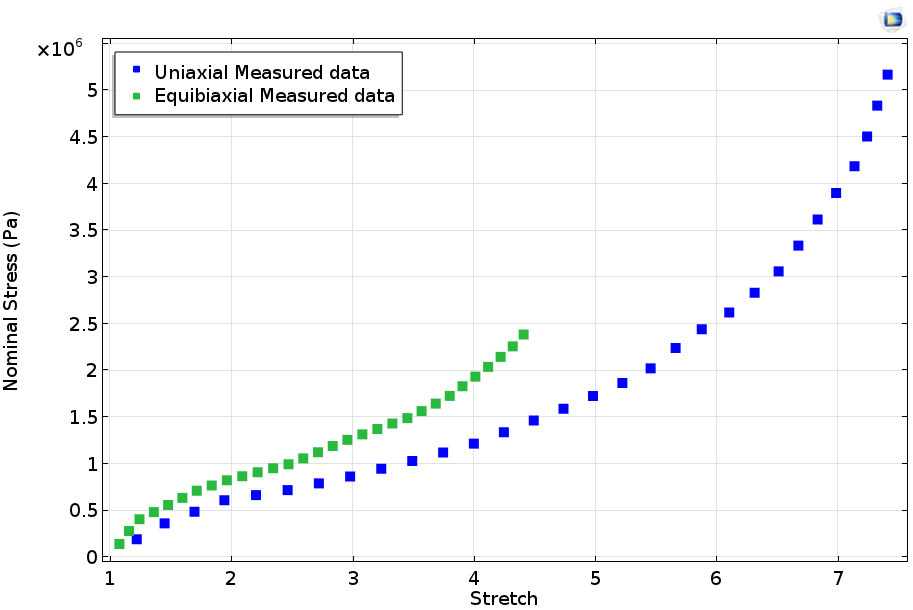
Measured stress-strain curves by Treloar.
Let’s begin by setting up the model to fit the uniaxial Neo-Hookean stress to the uniaxial measured data. The first step is to add an Optimization interface to a 0D model. Here, 0D implies that our analysis is not tied to a particular geometry.
Next, we can define the material parameters that need to be computed as well as the variable for the analytical stress versus stretch relationship. The screenshot below shows the parameters and variable defined for the case of an uniaxial Neo-Hookean material model.
")
Within the Optimization interface, a Global Least-Squares Objective branch is added, where we can specify the measured uniaxial stress versus stretch data as an input file. Next, a Parameter Column and a Value Column are added. Here, we define lambda (stretch) as a measured parameter and specify the uniaxial analytical stress expression to fit against the measured data. We can also specify a weighing factor in the Column contribution weight setting. For detailed instructions on setting up the Global Least-Squares Objective branch, take a look at the Mooney-Rivlin Curve Fit tutorial, available in our Application Gallery.
")
We can now solve the above problem and estimate material parameters by fitting our uniaxial tension test data against the uniaxial Neo-Hookean material model. This is, however, rarely a good idea. As explained in Part 1 of this blog series, the seemingly simple test can leave many loose ends. Later on in this blog post, we will explore the consequence of material calibration based on just one data set.
Depending on the operating conditions, you can obtain a better estimate of material parameters through a combination of measured uniaxial tension, compression, biaxial tension, torsion, and volumetric test data. This compiled data can then be fit against analytical stress expressions for each of the applicable cases.
Here, we will use the equibiaxial tension test data alongside the uniaxial tension test data. Just as we have set up the optimization model for the uniaxial test, we will define another global least-squares objective for the equibiaxial test as well as corresponding parameter and value columns. In the second global least-squares objective, we will specify the measured equibiaxial stress versus stretch data file as an input file. In the value column, we will specify the equibiaxial analytical stress expression to fit against the equibiaxial test data.
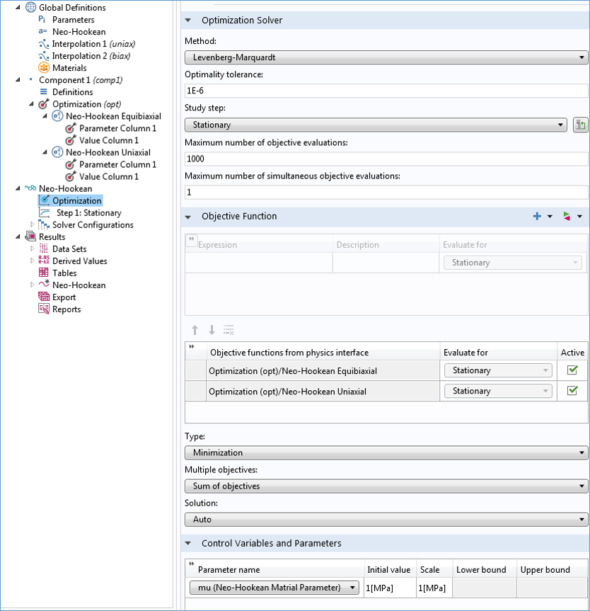
The settings of the Optimization study step are shown in the screenshot below. The model tree branches have been manually renamed to reflect the material model (Neo-Hookean) and the two tests (uniaxial and equibiaxial). The optimization algorithm is a Levenberg-Marquardt solver, which is used to solve problems of the least-square type. The model is now set to optimize the sum of two global least-square objectives — the uniaxial and equibiaxial test cases.
The plot below depicts the fitted data against the measured data. Equal weights are assigned to both the uniaxial and equibiaxial least-squares fitting. It is clear that the Neo-Hookean material model with only one parameter is not a good fit here, as the test data is nonlinear and has one inflection point.
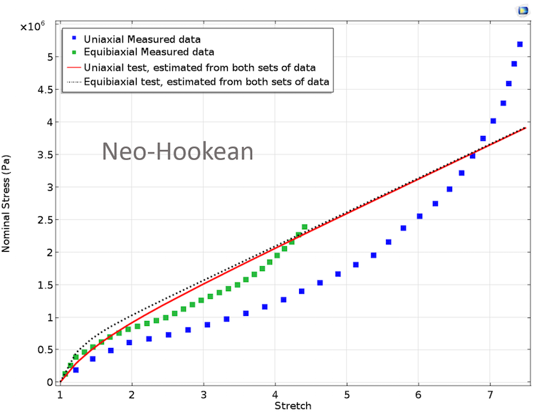
Fitted material parameters using the Neo-Hookean model. Equal weights are assigned to both of the test data.
Fitting the curves while specifying unequal weights for the two tests will result in a slightly different fitted curve. Similar to the Neo-Hookean model, we will set up global least-squares objectives corresponding to Mooney-Rivlin, Arruda-Boyce, Yeoh, and Ogden material models. In our calculation below, we will include cases for both equal and unequal weights.
In the case of unequal weights, we will use a higher but arbitrary weight for the entire equibiaxial data set. It is possible that you may want to assign unequal weights only for a certain stretch range instead of the entire stretch range. If this is the case, we can split the particular test case into parts, using a separate Global Least-Squares Objective branch for each stretch range. This will allow us to assign weights in correlation with different stretch ranges.
The plots below show fitted curves for different material models for equal and unequal weights that correspond to the two tests.
")
")
")
")
Left: Fitted material parameters using Mooney-Rivlin, Arruda-Boyce, and Yeoh models. In these cases, equal weights are assigned to both test data. Right: Fitted material parameters using Mooney-Rivlin, Arruda-Boyce, and Yeoh models. Here, higher weight is assigned to equibiaxial test data.
The Ogden material model with three terms fits both test data quite well for the case of equal weights assigned to both tests.
Fitted material parameters using the Ogden model with three terms.
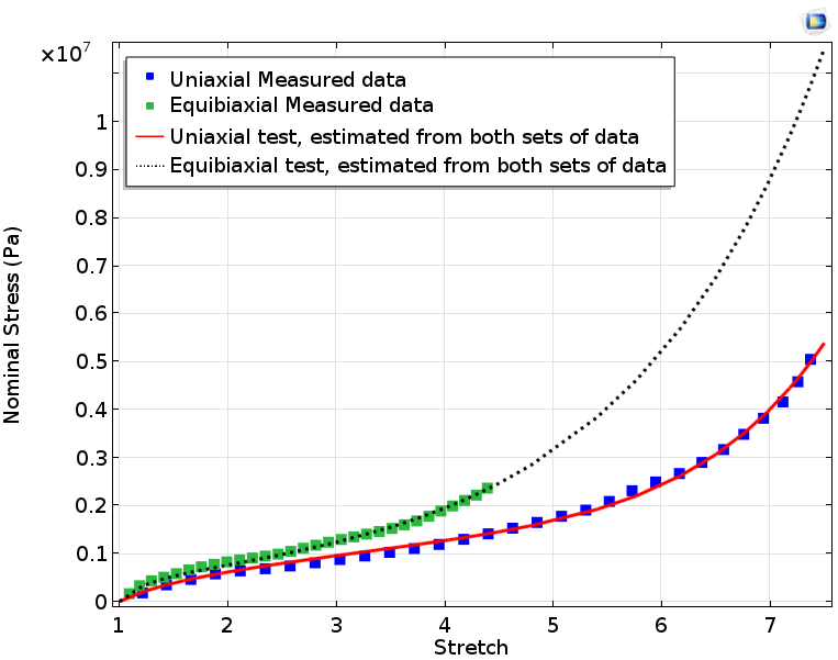
If we only fit uniaxial data and use the computed parameters for plotting equibiaxial stress against the actual equibiaxial test data, we obtain the results in the plots below. These plots show the mismatch in the computed equibiaxial stress when compared to the measured equibiaxial stress. In material parameter estimation, it is best to perform curve fitting for a combination of different significant deformation modes rather than considering only one deformation mode.
")
")
")
Uniaxial and equibiaxial stress computed by fitting model parameters to only uniaxial measured data.
Concluding Remarks
To find material parameters for hyperelastic material models, fitting the analytic curves may seem like a solid approach. However, the stability of a given hyperelastic material model may also be a concern. The criterion for determining material stability is known as Drucker stability. According to the Drucker’s criterion, incremental work associated with an incremental stress should always be greater than zero. If the criterion is violated, the material model will be unstable.
In this blog post, we have demonstrated how you can use the Optimization interface in COMSOL Multiphysics to fit a curve to multiple data sets. An alternative method for curve fitting that does not require the Optimization interface was also a topic of discussion in an earlier blog post. Just as we have used uniaxial and equibiaxial tension data here for the purpose of estimating material parameters, you can also fit the measured data to shear and volumetric tests to characterize other deformation states.
For detailed step-by-step instructions on how to use the Optimization interface for the purpose of curve fitting, take a look at the Mooney-Rivlin Curve Fit tutorial, available in our Application Gallery.

Comments (5)
Yi Luo
September 7, 2017Thank you so much for this post. It’s very useful for me.
Yi Luo
September 7, 2017Thank you so much for this post. It’s very useful to me.
Frido Hanl
June 21, 2018Thanks a lot for the post.
Maybe you’d like to correct a missing bracket in the uniaxial “Mooney-Rivlin, Five Parameters” equation.
Reinhard Wimmer
April 6, 2022Thanks for this great blog! But one question remains regarding Neo-Hookean Model. The shear modulus is equal to “mu” but in different other papers I read that this Neo-Hookean Parameter has to be multiplied by 2 (µ=2*C_10)? It is also stated on the Wiki-Page of Neo-Hookean Model?
Nora Asyikin Zulkifli
May 24, 2022Hi,
First of all, thank you for such an insightful and helpful post.
I do wonder though whether COMSOL has a built-in feature to check the Drucker’s stability?