

Dolphins and bats have relied on echolocation for millions of years. Yet, it would take until the early 1900s before humans first developed and used sonar. Not long after came the first countermeasure: the anechoic coating. Today, we’ll look at how you can model the reduction in echo that this provides using COMSOL Multiphysics®. Similar modeling techniques can also be used for other periodic structures, such as perforates, phononic crystals, and various sound absorbers.
Anechoic Coatings
To avoid detection by sonar during World War II, the German Navy covered their U-boats in rubber sheets with drilled air holes at regular distances. The same basic technology of embedding periodic patterns in spongy coatings is still in use, although the specifics are evolving. Finding the pattern and material properties that will minimize the echo for a desired range of frequencies is not an easy task, but one that lends itself very well to modeling.
Let’s find out how you can set up a model of an anechoic coating using the COMSOL Multiphysics® software. For our demonstration, we’ll consider a coating discussed in Ref. 1. The authors of this paper propose a quadratic array of tiny cylindrical holes stamped into a thin polydimethylsiloxane (PDMS) film. The film is placed on the submarine hull with the holes facing the steel. Hence, the holes form air bubbles, even when the vessel is submerged in water. Despite having a thickness of only 0.2 mm, this setup results in less than 10% reflectance for most of the frequency range between 1 and 2.8 MHz, and less than 50% reflectance all the way up to 5 MHz.
Finding the Smallest Unit Cell
When setting up models with periodic geometries, the first thing you want to figure out is how far you can reduce the size of the model geometry. The figure below shows the periodic pattern of air cavities. The blue dashed-line square indicates an obvious and completely general choice of unit cell. Flanked by periodic Floquet boundary conditions, this geometry would allow for incident radiation from an arbitrary angle. See our Porous Absorber model for an example of oblique incidence on a periodic structure.
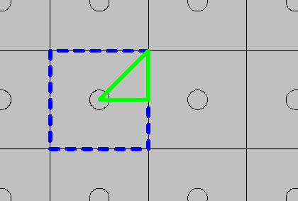
Top view of the periodic pattern with two candidate unit cells.
By assuming perpendicular plane wave incidence, we can exploit not only the periodicity, but also the geometric mirror symmetries. After establishing the x– and y-plane symmetries, it can be easy to forget that there is one mirror plane left, forming a 45-degree angle with both the x– and y-axes. This leaves us with the green solid-line triangle in the illustration, constituting 1/8 of the full periodic unit cell. Keep in mind, of course, that failing to notice and use a symmetry is not the end of the world — it merely makes the model more expensive than necessary to run.
Truncating the Geometry
Here is what the resulting geometry looks like, with water above the PDMS and steel below it:
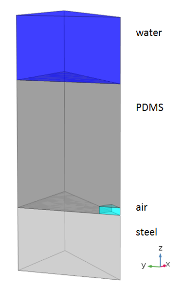
Model geometry produced in COMSOL Multiphysics® with the add-on Acoustics Module.
We will take both the steel and the water to continue indefinitely beyond the modeled geometry. While this is clearly a good assumption for the water, it may seem like a less than obvious choice for the steel. Outer submarine hulls can be just a few millimeters thick, and omitting the other side of the hull means neglecting any reflections that might occur on the inside.
However, the transmission into the steel is small because of the high acoustic impedance contrast between the PDMS and the steel. Also, much of the reflected sound would likely be absorbed by the coating. Therefore, including the full thickness of the steel domain is left as an exercise for the curious reader. If you try this, please tell us about it in the comments section!
Materials that go on “forever” can be modeled either with various low-reflecting boundary conditions or with perfectly matched layers (PMLs). The former work optimally under the assumption of perpendicular plane waves. PMLs are more general, making them the preferred choice in nonperiodic, open geometries. For more information on PMLs, see our blog post on perfectly matched layers for wave electromagnetics problems — the considerations and conclusions are similar in pressure acoustics and structural mechanics.
Diffraction
So, can we expect only perpendicular plane waves at the ends of our geometry? To know for sure, we need a primer on diffraction theory.
The transmitted and reflected waves caused by a plane wave incident on a periodic pattern can be described as a sum of plane waves propagating in a finite number of discrete diffraction angles. In the immediate vicinity of the pattern, you will, of course, also have some arbitrarily shaped evanescent fields. Nevertheless, the propagating waves are all plane.
Typically, most of the acoustic energy will end up in the “zeroth diffraction order”, which is just the refraction and mirror reflection of the incident wave. Reflected higher diffraction orders occur at angles where the path distance between radiation traveling in the same direction from two neighboring unit cells is an integer number of wavelengths. This happens according to the equation
Here, m = 0, +/-1, +/-2,.. is the diffraction order; ci is the pressure speed of sound in the incident medium; f is the frequency; d is the width of the repeating unit cell; θi is the angle of incidence; and θr,m is the angle of the mth order reflected diffracted wave.
Similarly, for the transmitted diffraction orders, we have
with ct being the pressure wave speed of sound in the final medium and θt,m the angle of the mth order transmitted diffracted wave.
Let us now look at the anechoic coating model, with θi = 0. For an mth order reflected diffracted wave to exist, we need
So, if c_i/(fd)>1, we have no reflected diffracted waves. In the same manner, provided c_i/(fd)>{c_i/c_t}, we have no transmitted diffraction orders. The pressure speed of sound is higher in steel than in water, so diffraction would arise in the reflected waves first. With d = 120 µm and ci = 1481 m/s, we can finally conclude that there is no diffraction at frequencies below 12.3 MHz.
Setting up the Anechoic Coating Model
Having decided that PMLs are not required in the relevant frequency spectrum, we need only leave a sufficient depth of water and steel in the model so that most of the evanescent wave content will have died out before reaching the exterior boundaries. For boundary conditions, we use a Low-Reflecting Boundary in the steel and the pressure acoustics counterpart, Plane Wave Radiation, in the water.
Speaking of Pressure Acoustics, that interface applies both in the water and in the air cavities. When modeling small confined spaces, the Thermoviscous Acoustics interface can be worth considering as a potentially more accurate option. However, it is only needed if the thermal and/or viscous boundary layers have a significant thickness. At the frequencies that we are concerned with here, these layers do remain much thinner than the dimensions of the cavity.
The steel and PDMS domains are modeled with Solid Mechanics. If you select Acoustic-Solid Interaction, Frequency Domain in the COMSOL Multiphysics® Model Wizard, you get the two relevant interfaces and an Acoustic-Structure Boundary automatically connecting them together.
The model is excited with an incident perpendicular wave added to the plane wave radiation condition. To find out the transmission, reflection, and absorption coefficients, you need to extract what fraction of the energy is passing through, being reflected, and being absorbed, respectively.
The transmitted power is simple. The outward mechanical energy flux is automatically available as solid.nI, so all you need to do is integrate that over the low-reflecting boundary terminating the steel domain. Divide that by the incident power, which for a plane wave has a known analytical expression, and you achieve the transmission coefficient.
The net acoustic intensity comes as a vector (acpr.Ix, acpr.Iy, acpr.Iz). To get the reflected power, take the negative of the z-component and subtract its integral over the inlet from the incident power. Divide by the incident power again and you have the reflection coefficient. Finally, the absorption coefficient is most conveniently achieved from the condition that all three coefficients sum up to 1.
Results
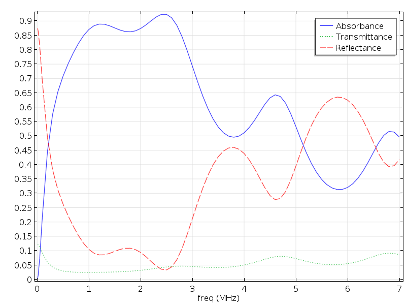
The below plot shows the resulting transmission, reflection, and absorption coefficients. The results are generally in good agreement with those in the paper (referenced at the end of this post).
Further Resources
- Look at other acoustics models and apps with periodic geometries:
- Read related blog posts:
- Learn about the transfer impedance of a perforate
- Another blog post on modeling an RF anechoic chamber discusses similar techniques applied to electromagnetic waves
Reference
- V. Leroy, A. Strybulevych, M. Lanoy, F. Lemoult, A. Tourin, and J. H. Page: Superabsorption of acoustic waves with bubble metascreens, Phys.Rev. B 91, 020301(R), 2015

Comments (1)
David Wang
March 22, 2020Dear Linus Andersson,
I set my own simulation like the case model, but once I set the hydrostatic pressure in the interface between water and rubber(just like PDMS in the case model), the result of sound absorption is negative (-)…I want to know How To Add Hydrostatic Pressure To such case.