

When modeling acoustics phenomena, particularly of devices with small geometric dimensions, there are many complex factors to consider. The Thermoviscous Acoustics interface offers a simple and accurate way to set up and solve your acoustics model for factors such as acoustic pressure, velocity, and temperature variation. Here, we will demonstrate how to model your thermoviscous acoustics problems in COMSOL Multiphysics and provide some tips and resources for doing so.
Considerations for Modeling Thermoviscous Acoustics
When modeling acoustics phenomena using the Thermoviscous Acoustics interface, you first need to set up your physics correctly, where the mesh has to resolve the viscous and thermal boundary layers. It is also important to note that solving a thermoviscous acoustic model involves solving for the acoustic pressure; velocity field (for example, 3 components in 3D); and temperature variations. For this reason, your acoustics models may become computationally expensive and involve many degrees of freedom (DOFs) — meaning a longer wait for your results.
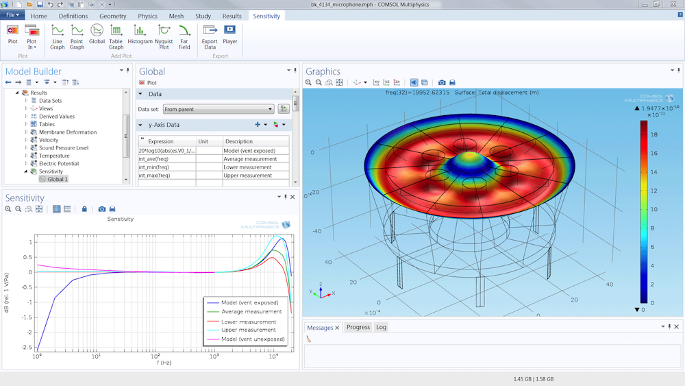
A condenser microphone is a common application of thermoviscous acoustics modeling.
One common problem mentioned in COMSOL Multiphysics support cases for acoustics simulation is the erroneous specifications of the coefficients of thermal expansion \alpha_0 and isothermal compressibility \beta_\textrm{T}. If these coefficients are incorrect or evaluate to zero, the resulting model will contain acoustic waves (pressure or compressibility waves) that propagate at the wrong speed of sound or do not propagate at all. The speed of sound c relates to both of these coefficients through
where \rho_0 is the background density, T_0 the background temperature, and C_\textrm{p} the heat capacity at constant pressure.
A detailed description of both of these coefficients and how to define them is given in the User’s Guide for the Acoustics Module, under the section on the Thermoviscous Acoustics, Frequency Domain interface in the Thermoviscous Acoustics Model section. The Vibrating Particle in Water — Correct Thermoviscous Acoustic Material Parameters tutorial model, found in the Application Library, also discusses these issues.
A simple method for checking your coefficients is to plot the parameters ta.betaT (isothermal compressibility) and ta.alpha0 (thermal expansion) after solving the model to ensure that they have the correct values.
Meshing Thermoviscous Acoustics Models
When meshing a thermoviscous acoustics model, it is important to properly resolve the acoustic boundary layer to capture the physics correctly. In order to do this, as well as to avoid too many mesh elements, there are a few tricks you can use, for instance, by creating parameters to control your mesh. You can create a parameter for the analysis frequency, say f0, and then also create a parameter for the viscous (or thermal) boundary layer thickness at this frequency. In air, we know that the viscous boundary layer thickness at 100 Hz is 0.22 mm, and, in general, you can write the thickness as dvisc = 0.22[mm]*sqrt(100[Hz]/f0). If you perform a frequency sweep, you can create parameters for the thickest and thinnest value of the boundary layer. Having these parameters at hand can help you build a good mesh.
Another tip to remember for meshing your thermoviscous acoustic model is to use boundary layers. This will keep the number of mesh elements constant for all studied frequencies. This is especially important for a 3D geometry. If you simply prescribe a maximum element size on the walls, the number of mesh elements will explode as the boundary layer thickness decreases.
When defining the mesh, also be sure to use logic expressions. For example, use min(,) when defining the maximum element size or the thickness of a boundary layer. The figure below shows a circular duct with a diameter 2a = 2 mm. The overall Maximum element size is set to a/3. A boundary layer mesh is used with five layers and a thickness of min(a/30,0.3*dvisc). This ensures a constant mesh thickness of up to around 500 Hz (to maintain a quality mesh in the center of the pipe). Then, the thickness decreases with dvisc as the frequency parameter f0 increases.
In general, when solving a model using the Frequency Domain study step, it is not possible to have the mesh depend on the frequency variable freq. However, it is possible to achieve this when performing a parametric sweep. Therefore, one workaround is to use a parametric sweep around the Frequency Domain study step. Sweep the parameter over f0 and set f0 to be the frequency in the Frequency Domain step.
Note that when performing a parametric sweep, COMSOL Multiphysics will remesh every time a parameter in the mesh changes, which may noticeably slow down the computation. On the other hand, because you can set up a more optimized mesh this way, you can still save time.
A final option is to prepare several meshes — maybe one mesh for each chunk of 1000 Hz — and then use several studies with these meshes selected for a restricted frequency range.
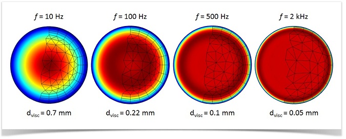
A mesh that captures the effects in the acoustic boundary layer, shown here at four different frequencies. The color represents the RMS velocity for a wave traveling in an infinite circular duct with a diameter of 2 mm.
Keeping Your Simulation Computationally Efficient
Because it is so computationally expensive to solve thermoviscous acoustics models, it is usually advantageous to do so only in the components of your system where this type of physics is relevant. These simulations can then be combined with simulations based on less complex physics that describe the rest of your system. Let’s see how you can apply this tactic to your own simulation work.
One option is to couple your thermoviscous acoustics model to pressure acoustics, where relevant. In models where large differences exist in the geometry scale, use thermoviscous acoustics in only the narrow regions and use pressure acoustics for the larger domains. The Thermoviscous Acoustics interface is a multiphysics interface that has the ability to be automatically coupled to the Pressure Acoustics interface, making this process seamless. This is demonstrated in detail in the Generic 711 Coupler tutorial model.
You can also use submodels and lumped models in an effort to conserve your thermoviscous acoustics modeling efforts. For instance, you can extract a transfer impedance from a detailed thermoviscous acoustic model and use it in a pressure acoustics model. A tutorial model that exemplifies this process is the Acoustic Muffler with Thermoacoustic Impedance Lumping. In this example, the transfer impedance of a perforated plate is analyzed and used in a pressure acoustics model. Also note that as the frequency of your model increases, the acoustic boundary layer decreases in size and relevance. This means that at a certain frequency, the boundary layer losses can be considered negligible, and you can switch to solving the model as a pressure acoustics problem.
When modeling structures of constant cross section, you can use the Narrow Region Acoustics models in the Pressure Acoustics interface. These are homogenized fluid models where the boundary layer losses are smeared over the width of the fluid domain (homogenized). In ducts with constant or slowly varying cross sections, this model gives a correct distribution of losses along the length of the duct. In other cases, these models provide a good first approximate response of a system without the computational cost of solving a full thermoviscous acoustic model. See the Lumped Receiver Connected to Test Set-up with a 0.4cc Coupler tutorial model to learn how to use the Narrow Region Acoustics models.
If the model becomes very large, you can also turn to the documentation for the Thermoviscous Acoustics interface, which contains even more tips and tricks for how to use different solver approaches and remedy this issue. Go to Acoustics Module User’s Guide > Thermoviscous Acoustics Interfaces > Modeling with the Thermoviscous Acoustics Branch > Solver Suggestions for Large Thermoviscous Acoustics Models for more information.
Concluding Thoughts on How to Model Thermoviscous Acoustics
The most important guidelines to consider when using the Thermoviscous Acoustics interface include:
- Solve only for thermoviscous acoustics where and when necessary. Investigate if the viscous and/or thermal boundary layer thicknesses are comparable to the geometrical scale (depending on the frequency range and geometry scales).
- Check your material parameters to be sure that both compressibility and thermal expansion are nonzero.
- Check your mesh size at the boundaries and compare it to the viscous and thermal boundary layer thicknesses.
Application Examples
These tutorial models demonstrate step-by-step how to simulate thermoviscous acoustics systems, covering a wide range of application areas.
- Axisymmetric Condenser Microphone
- The Brüel & Kjær 4134 Condenser Microphone
- Vibrating Micromirror with Viscous and Thermal Damping
- Acoustic Muffler with Thermoacoustic Impedance Lumping
- Generic 711 Coupler — An Occluded Ear Canal Simulator
- Photoacoustic Resonator
- Vibrating Particle in Water — Correct Thermoviscous Acoustic Material Parameters
- Energy Conservation with Thermoacoustics
Further Reading and References
- Check out the previous blog post in this series: Theory of Thermoviscous Acoustics: Thermal and Viscous Losses
- Find a detailed demonstration on how to analyze thermoviscous acoustics in a microphone
- Learn how to model a MEMS microphone using COMSOL Multiphysics
- Read the Thermoviscous Acoustics Interfaces section of the Acoustics Module User’s Guide included with the COMSOL documentation
Editor’s note: This blog post was updated on 7/12/16 to be consistent with version 5.2a of COMSOL Multiphysics.


Comments (0)