
The Octave Band plot provides you with an easy and flexible way to represent simulation results that are essential when modeling acoustics applications, including frequency responses, transfer functions, sensitivity curves, transmission losses, and insertion losses. Let’s learn a bit more about the Octave Band plot while highlighting its various options and settings.
Editor’s note: The original version of this post was published on January 21, 2016. It has since been updated to reflect new features and functionality available in the Acoustics Module.
The Importance of Octaves
When discussing an octave, we are referring to a frequency band in which the upper frequency is twice the lower frequency. Applying this concept results in bands of equal width on a logarithmic frequency axis.
Representing an acoustic response by binning the signal energy into octaves, or fractional octaves, is very common for acoustic and audio engineers. This visualization technique is closely related to specifications in standards and, thus, the way measurement equipment works (e.g., sound level meters). Physiologically, such representation is motivated by the fact that the human ear itself filters (via auditory filters) and perceives sound on a logarithmic frequency scale. In the same way, the human ear also has a logarithmic sensitivity to sound magnitude, hence the use of a decibel (dB) scale for sound pressure levels.
As we will describe next, the Octave Band plot includes more functionality than simply plotting acoustic responses in octave bands.
The Octave Band Plot, a Simple and Versatile Acoustics-Specific Plot
The Octave Band plot, available in the Acoustics Module add-on to COMSOL Multiphysics®, includes built-in features specific to acoustics simulations that can be helpful for representing and analyzing frequency-domain data. The output of the plot is automatically given on the dB scale, with several formatting options. With regards to the data fed to the plot, you can use any global quantity, or readily pick it up at a point or as an average over a line, surface, or volume.
For the graphs, you have the option to format the results so that they render in either bands (octaves, 1/3-octaves, or 1/6-octaves) or as a continuous curve. The band format can represent the band power or band-average power spectral density (PSD), while the continuous curve represents PSD data. You can also easily add weighting to the response curve, with the choice of a Z-, A-, C-, or user-defined weighting. For the input to the plot, you can modify it to represent amplitude (e.g., the absolute value of a pressure), power (e.g., the power of incoming or outgoing modes at ports or an intensity integrated over a surface), or a general transfer function.
All of these options help to simplify postprocessing considerably. Furthermore, this plot type makes it much easier to compare results with measured data, which is often given in octave or 1/3-octave bands.
The screenshot below shows the user interface (UI) for the Octave Band plot. In the next section, we will explain its different options and settings in detail.

The UI for the Octave Band plot.
An Overview of the Different Options and Settings
Geometric Entity Level
The Geometric entity level drop-down menu enables you to select how the input data is picked up from the model. The data can be directly taken from a point in the model if, perhaps, a sensitivity is measured at a specific location. By selecting Edge, Boundary, or Domain, the input is automatically averaged. When averaging, the pressure or power is averaged before transformation to the dB scale. Such an approach is useful, for example, when calculating the response in an ear simulator. Here, the average pressure is easily picked up on the measurement microphone surface. Thus, it is not necessary to set up integration or average operators nor perform a surface average in an Evaluation Group.
The Geometric entity level selection can also be used to evaluate global quantities. You could, for example, evaluate the pressure in a point outside of the computational domain using the Exterior Field Calculation feature operator.
Expression Type
With the Expression type selection (in the y-Axis Data section), you can decide how the input data in the Octave Band plot is interpreted. There are three available options: Amplitude, Power, and Transfer function.
The default option is Amplitude. When this is selected, the input in the Expression field is treated as a complex amplitude, p, which is most often the pressure in acoustics applications. The entered value is then used to evaluate the level as
where the RMS pressure is calculated as p_\textrm{rms}^2 = 0.5 |p|^2. The reference pressure, p_\textrm{ref}, is entered into the Amplitude reference field and is assumed to be a RMS quantity. In most acoustics interfaces, the default value is phys.pref_SPL, which is defined in the sound-pressure-level settings at the physics interface level. The default value is typically 20 \mu Pa. As an example, when defining a transfer function, the reference amplitude could be set to the RMS amplitude, 1/\sqrt{2}\:\textrm{Pa}, of an incident plane wave that has a peak amplitude of 1\:\textrm{Pa}, and the input in the Expression field could be the average pressure measured over a surface.
The next option is Power. Here, the input to the plot entered into the Expression field is assumed to be a power, P. The value could be calculated, for example, from an integral of the acoustic intensity over a surface. The level is computed as
where the reference power, P_\text{ref}, is entered into the Power reference field. The default is phys.Pref_SWL, which is the reference sound power level of 10^{-12} \: \textrm{W}.
Transfer function is the final option. Any user-defined transfer function, H, and a reference level, L_\textrm{ref}, can be entered in this case. They are used to define the level
The input data is used to integrate the power within bands when the results are plotted as octave, 1/3-octave or 1/6-octave bands, depending on the style that you choose.
Plot Quantity and Weighting
Under the Plot selection, there are two drop-down menus that offer you different choices for formatting your data. These are the Quantity and the Weighting drop-down menus.
Using the Quantity drop-down menu, you can plot the frequency-domain data as either Continuous power spectral density, Band power, or Band average power spectral density. The choice of band power versus band-average PSD determines how the band power summation and averaging is performed. When either of the band options is selected, you can choose the Band type as Octave, 1/3 Octave, or 1/6 Octave. Finally, there is an option, Use in-band data only, that can be selected (the default) or deselected. When this option is selected, only data points lying inside a given band are used for the integration and interpolation of data. This option typically has an influence on results for data with low resolution (i.e., only a few points in each band).
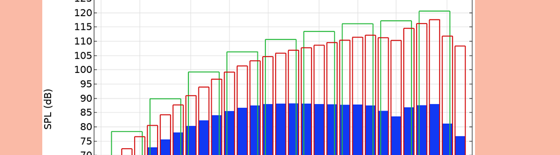
Three different plot styles are highlighted in the figure below. The bars outlined in red indicate the 1/3-octave band power data, the bars outlined in green indicate the octave band power data, and the solid blue bars represent the 1/3-octave band-average power spectral density (PSD) data. (The formatting of the bars can be changed via the Coloring and Style section.) The plot is a modified version of the one from our Loudspeaker Driver tutorial model.
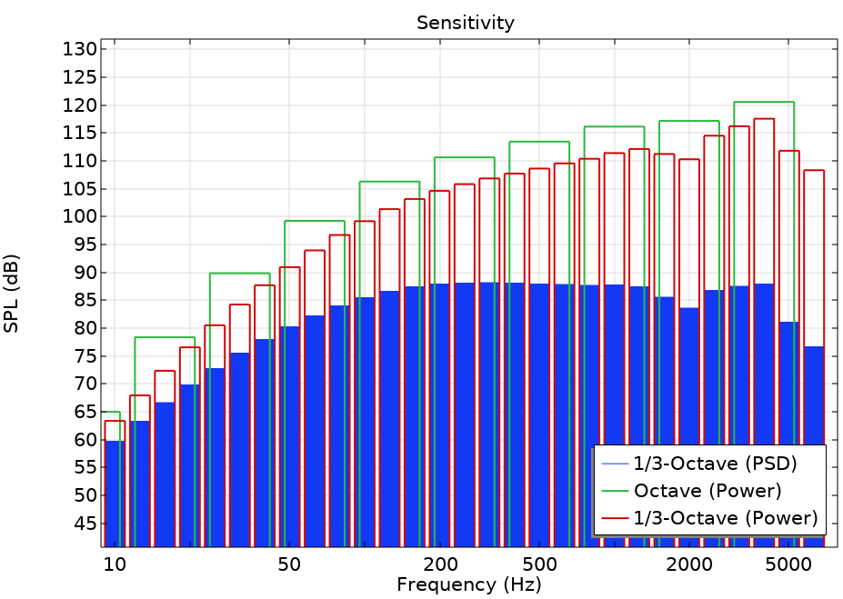
A graph depicting the different plot styles.
Lastly, using the Weighting selection, you can identify the weighting that should be applied to the data. The choices include:
- Z-weighted (flat): Zero weighting is applied (the default option).
- A-weighted: The IEC 61672-1 standard A-weighting is applied to the data. It is used to account for the perceived loudness of the human ear.
- C-weighted: The IEC 61672-1 standard C-weighting is applied to the data. This option can also account for the perceived loudness of the human ear, usually for very loud levels of noise.
- Expression: A user-defined value or expression is used for the weighting. In the Expression field, an expression that defines the gain as a function of the frequency,
freq, is entered. The gain provided in dB is then given as20·log10(expression).
The two curves in the figure below represent the A- and C- weights applied to a flat, 0-dB response. A user-defined linear weighting is given as 10^{-3}\cdot f and is represented in 1/3-octave bands (shown in red).
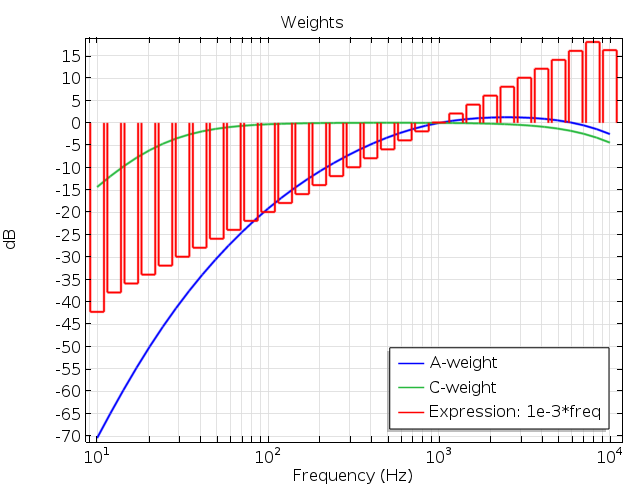
A plot showing the different weighting options.
Using an Octave Band Plot: An Absorptive Muffler Example
The Absorptive Muffler tutorial model (located in the Acoustics Module > Automotive folder within the Application Libraries) uses the Octave Band plot to depict the transmission loss of a muffler system. In this version of the model, the Transfer function option is selected for the Expression type. The input to the plot is the ratio of the total incident power to the total transmitted power. These elements are calculated by using the built-in variables for the power of incident and outgoing modes at the Port conditions.
For pure plane-wave propagation (below about 2500 Hz), there is another way to plot the transmission loss without using the port power variables. To do so, you set the Geometric entity level to Boundary and select the outlet boundary number 28. In the Expression field, enter p_in (the amplitude of the incident plane wave), and in the Amplitude reference field, enter sqrt(0.5)*acpr.p_t. Remember, it is assumed that the reference is a RMS value, hence, the sqrt(0.5) factor is needed (as seen in the screenshot below). Choosing the Continuous power spectral density plot style and clicking on the Plot button gives the results shown below for the case of a muffler with the liner.
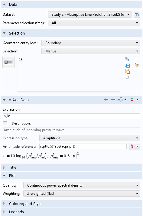
Plot settings for the Octave Band plot for the absorptive muffler.
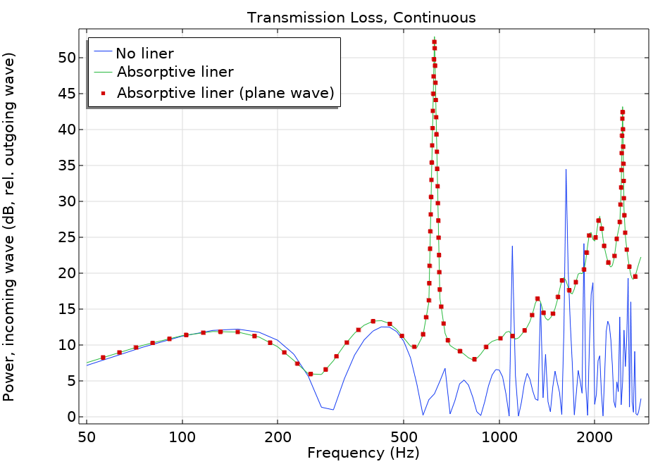
Transmission loss comparison plot for the absorptive muffler.
Explore Octave Band Plots with These Resources
In addition to the example referenced above, you can find many other tutorial models in the Application Libraries that utilize the Octave Band plot. We’ve listed a few of these tutorial models here, all of which are available for download from our Application Gallery.
- Loudspeaker Driver
- Lumped Loudspeaker Driver
- The Brüel & Kjær 4134 Condenser Microphone
- Loudspeaker Driver in a Vented Enclosure
Reference
- IEC 61672-1 Electroacoustics — Sound level meters — Part 1: Specifications.


Comments (8)
Ian Chou
August 21, 2019Hi
Why this (where the rms pressure is calculated as prms^2=0.5|P|^2) ?
Mads Herring Jensen
August 26, 2019 COMSOL EmployeeHi Ian
This is the definition of an RMS value. The RMS value of a harmonic signal is given by sqrt(0.5)*abs(p), where abs(p) corresponds to the peak value. We work in the frequency domain so all signals are harmonic. The SPL is defined in the standards through the RMS pressure values.
Best regards, Mads
Ysbrand Wijnant
February 28, 2020Dear Mads,
I truly believe this is a wrong implementation.
Energetically adding 3 1/3-octave band values within an octave band, always results in the octave value being larger than the largest 1/3-octave value. It seems you are averaging the values but this is incorrect, irrespective of the type of sound. (see also http://www.sengpielaudio.com/calculator-octave.htm)
Best regards,
Ysbrand
Mads Herring Jensen
March 2, 2020 COMSOL EmployeeDear Ysbrand, The plot is not adding 1/3 octaves to get the octave values. The plot simply filters the continuous response curve into octaves or 1/3 octaves (integrating the power in these bands). The input to the model is not a filtered signal, it is a continuous spectrum. If you use the dynamic help (press F1) when you have selected the Octave Band plot in the UI, you will get the following explanation: “An octave band plot corresponds to plotting the average or integrated value of, for example, the squared pressure over a given frequency band defined by the center frequency or midfrequency and the bandwidth. What the plot shows is a “white noise transfer function” of the system; that is, it assumes that the input is of the same nature as the output.” Best regards, Mads
Ysbrand Wijnant
March 10, 2020Dear Mads,
Thanks for the reply. I am a bit confused now as the integration of power in the 3 1/3 octave bands (making the the octave band) will still give you a value which is higher than the highest 1/3 octave band value. So filtering should indeed give a higher value and this is not what I see in the results. Maybe I am wrong but the implementation is, to my knowledge, not consistent to how octave bands are usually used (and why they are used) and implemented.
Best regards,
Ysbrand
Jobin Puthuparampil
December 6, 2021Hey Mads, like Ysbrand above, I would appreciate further clarification on the implementation. I echo his questions.
Mads Herring Jensen
December 6, 2021 COMSOL EmployeeDear Jobin, please see my reply to Ysbrand. Best regards, Mads
Mads Herring Jensen
December 6, 2021 COMSOL EmployeeDear Ysbrand
In the upcoming release we have clarified the settings and added one more option. What we had implemented so far was the power spectral density in the bands and the continuous power spectral density. In version 6.0 we also have an option for the total power in the bands. This is probably the option you are looking for.
Best regards
Mads