

In Part 1 of this blog series, we discussed some of the considerations that you need to make when transforming your measured material data into a constitutive model. Hyperelastic materials were discussed in some detail. Today, we will have a look at how to use nonlinear elastic and elastoplastic materials, and show one way in which you can use your measured data directly in COMSOL Multiphysics.
Nonlinear Elastic Materials
Some materials already exhibit significant nonlinearity at small strains. Cast iron and some ceramics show this behavior, for example. However, when unloaded from a moderate strain, they follow the same stress-strain path back to the original state, so the response is elastic. This calls for a nonlinear elastic model.
In the previous blog post, we discussed hyperelastic materials, so why not just use one of these models to fit the measured stress-strain curve for, say, a nodular cast iron? The answer is that the hyperelastic material models are tailored for large strains. In elastomers, you may have elongations of several hundred percent of the original length, whereas the elastic range of metals and more brittle materials is usually less than 1%.
The very popular Mooney-Rivlin model will, for example, be essentially linear for small strains, and is therefore not useful in this context. In the Ogden model, the stress is computed as a sum of powers of the stretches. But for small strains, the stretch may have a range from 0.999 to 1.001 or so. In order to predict a significant nonlinearity, the exponent in the power law would have to be extremely high. A stable fitting of data to such an equation is not feasible. At the low strains present in a brittle material, the engineering strain would be a more natural representation of deformation. You can read more about different stress and strain measures in the blog entry “Why All These Stresses and Strains?”
To cope with this situation, COMSOL provides a set of nonlinear elastic models intended for small strains. These material models require the Nonlinear Structural Material Module or the Geomechanics Module and are available in the Solid Mechanics and Membrane interfaces. Let’s investigate how you can use these materials.
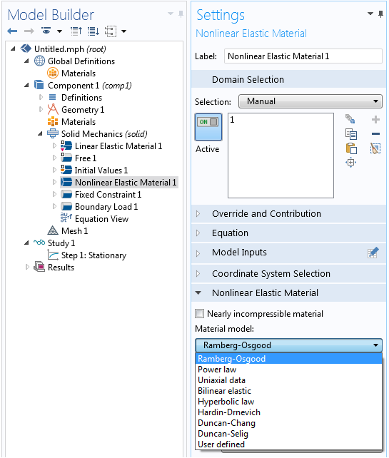
Selecting a nonlinear elastic material model in COMSOL Multiphysics.
In total, there are nine nonlinear elastic material models. Some of them have a simple mathematical form determined by a few parameters. One material model is especially useful when dealing with experimental stress-strain data: Uniaxial data. This model is explicitly intended for analyses based on measured data. Let’s have a look at the settings for this model:
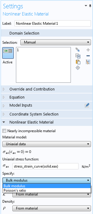
The settings for the Uniaxial data nonlinear elastic model.
The main input is a function relating the uniaxial stress to the uniaxial strain. In this example, the measured data is given in terms of an interpolation function, called stress_strain_curve, but it could also have been an analytical expression. An interpolation function can be entered explicitly as a number of data points or it can be read from a file. Here, the import is made directly from an Excel® file. This requires the LiveLink™ for Excel® add-on, but it is also possible to read the data from tabulated text files.
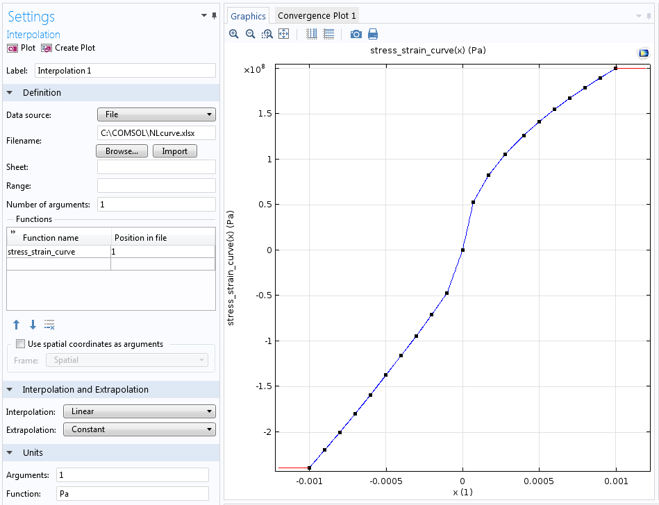
Imported uniaxial stress-strain curve.
The uniaxial curve does not, however, provide enough information to completely define a multiaxial constitutive law. One more assumption is needed, which is why you have to provide either a constant Poisson’s ratio or bulk modulus. For many materials, a constant Poisson’s ratio with a value between 0.2 and 0.3 will provide a good approximation. This is all that is needed to complete the material model.
If you study the stress-strain curve above, you will notice that it is different in tension and compression. In a multiaxial stress state, however, a certain point in the material may experience tension in one direction and compression in another. So which branch of the material curve should then be used? The material model is isotropic, so it has the same stiffness in all directions, but it is the volume change that is decisive. If the local volume change is negative, the compression branch is used.
Some Notes on the Theory
An isotropic nonlinear elastic material is only admissible from the theoretical point of view if:
- The mean stress (“pressure”) or bulk modulus is a function only of the volumetric strain.
- The shear stress or shear modulus is a function only of the shear strains.
If these conditions are violated, you can devise a stress-strain cycle from which it is possible to extract energy, that is, a perpetuum mobile.
All of the built-in materials are designed so that these conditions are fulfilled. If you take a look at the settings for the Bilinear elastic material, you will have to input the bulk moduli for this in tension and compression — not the Young’s moduli as you might have anticipated.
Most structural analysts work with Young’s modulus and Poisson’s ratio as the primary parameters for elastic materials. But the requirements above unfortunately mean that if Young’s modulus has a dependence on the strain, then…
- The function describing this dependency can only have some very specific forms.
- Poisson’s ratio must also be a function of strain, which leads to a function that is very difficult to express.
So how was it possible to enter the Uniaxial data above with a constant Poisson’s ratio? The answer is that we created behind-the-scenes allowable functions for the bulk modulus and shear modulus. No reference is made to Young’s modulus, even though that is what you would intuitively derive in the graph.
That said, I have seen quite a number of successful models where an analyst has introduced strain dependencies in the Young’s moduli for isotropic or orthotropic materials in an elastic material model. For practical engineering use, this may work fine. We supply an example of how to define a stress-dependent Young’s modulus in the Modeling Stress-Dependent Elasticity tutorial. The important point for such an approach to be acceptable is that the structure should be subjected to a mainly proportional loading (in the sense that the directions of the principal strains do not rotate).
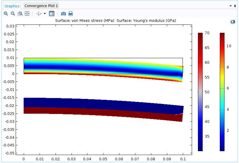
Cantilever beam with different values of Young’s modulus in tension and compression. The beam is subjected to a bending moment at the free end. The upper plot shows von Mises stress; the lower plot shows the current value of Young’s modulus.
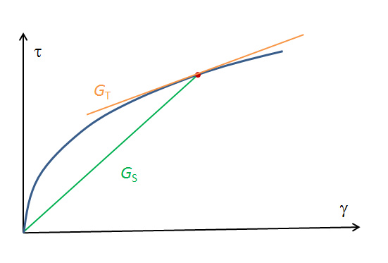
When you set out to model nonlinear elasticity by either using the built-in models or by your own expressions, it is important to keep a clear distinction between a tangent stiffness and a secant stiffness. A nonlinear elastic model is often expressed similarly to the linear model, but with a stress or strain dependence in the elastic constant (which is no longer a constant!). Assume that the shear stress \tau is related to the shear strain \gamma through
The shear modulus G_S(\gamma) is then a secant shear modulus. When the total strain is multiplied by the secant modulus, the result is the total stress. The tangent shear modulus G_T(\gamma), on the other hand, is the stiffness experienced for a small change in strain, as illustrated by the figure below.
Mathematically, the relation between the two moduli is
Your measured data will usually have the form
This means that the secant stiffness actually is
When converting a stress-strain curve into secant form using this expression, special attention must be given to the possible zero-divide at zero strain.
Also, you may sometimes encounter the statement that a certain material has been fitted to a power law with a certain exponent n. This may either mean that
or that
The Power law model in COMSOL Multiphysics uses the former, more common definition, where the strain exponent n relates to the slope of the stress-strain curve in a semi-log plot.
Approximating Plasticity with Nonlinear Elasticity
A pure tension experiment cannot determine whether a certain measured nonlinearity is caused by plasticity or not. The unloading curve must also be investigated. This is illustrated by the animation below, taken from the previous blog post.
The use of a nonlinear elastic model to simulate plasticity has been explored in a previous blog post.
In addition to using the Uniaxial data model, the Ramberg-Osgood nonlinear elastic material model is specifically intended for use as a simple replacement for a full elastoplastic model. Using a nonlinear elastic material is significantly cheaper in terms of computer resources, but what are the limitations of such an approach?
- Obviously, only a continuous increase in the loading is allowed.
- If there are several external loads acting, for example a pressure load together with thermal expansion, these are usually not proportional to each other. This may cause the local stresses to be non-proportional.
- The three-dimensional response will usually not be the same, even if the uniaxial stress-strain curve is identical for a nonlinear elastic model and a full elastoplastic model. In metal plasticity, like a von Mises flow rule, plastic deformation preserves the volume. This will not be the case in a corresponding nonlinear elastic model.
Concluding Remarks
When deciding upon a suitable material model, you must take into account the accuracy of the whole analysis. In engineering, we are often working with incomplete information, and there will be uncertainties in the loads, in the homogeneity of the materials, and in the actual dimensions of the structure. You will also introduce approximations by the selection of boundary conditions. It is the weakest link in the chain that determines the quality of the results, and that may well not be the exact mathematical foundation of the material model.
In the previous blog post, I stated that “it is not a good idea to just enter a simple stress-strain curve as input.”
So why did I change my mind today? The answer is that when working with the Uniaxial data model, it is the actual measurements that are used. For all hyperelastic models, and most of the other nonlinear elastic models, the measured data must be fitted to a mathematical model with a small number of parameters. It is this fitting that cannot safely be done without human supervision.

Comments (0)