

How do we check if a simulation tool works correctly? One approach is the Method of Manufactured Solutions. The process involves assuming a solution, obtaining source terms and other auxiliary conditions consistent with the assumption, solving the problem with those conditions as inputs to the simulation tool, and comparing the results with the assumed solution. The method is easy to use and very versatile. For example, researchers at Sandia National Laboratories have used it with several in-house codes.
Verification and Validation
Before using a numerical simulation tool to predict outcomes from previously unforeseen situations, we want to build trust in its reliability. We can do this by checking whether the simulation tool accurately reproduces available analytical solutions or whether its results match experimental observations. This brings us to two closely related topics of verification and validation. Let’s clarify what these two terms mean in the context of numerical simulations.
To numerically simulate a physical problem, we take two steps:
- Construct a mathematical model of the physical system. This is where we account for all of the factors (inputs) that influence observed behavior (outputs) and postulate the governing equations. The result is often a set of implicit relations between inputs and outputs. This is frequently a system of partial differential equations with initial and boundary conditions that collectively are referred to as an initial boundary value problem (IBVP).
- Solve the mathematical model to obtain the outputs as explicit functions of the inputs. However, such closed form solutions are not available for most problems of practical interest. In this case, we use numerical methods to obtain approximate solutions, often with the help of computers to solve large systems of generally nonlinear algebraic equations and inequalities.
There are two situations where errors can be introduced. First, they can occur in the mathematical model itself. Potential errors include overlooking an important factor or assuming an unphysical relationship between variables. Validation is the process of making sure such errors are not introduced when constructing the mathematical model. Verification, on the other hand, is to ascertain that the mathematical model is accurately solved. Here, we are ensuring that the numerical algorithm is convergent and the computer implementation is correct, so that the numerical solution is accurate.
In brief, during validation we ask if we posed the appropriate mathematical model to describe the physical system, whereas in verification we investigate if we are obtaining an accurate numerical solution to the mathematical model.
")
A comparison between the processes of validation and verification.
Now, we will dive deeper into the verification of numerical solutions to initial boundary value problems (IBVPs).
Different Verification Approaches
How do we check if a simulation tool is accurately solving an IBVP?
One possibility is to choose a problem that has an exact analytical solution and use the exact solution as a benchmark. The method of separation of variables, for example, can be used to obtain solutions to simple IBVPs. The utility of this approach is limited by the fact that most problems of practical interest do not have exact solutions — the raison d’être of computer simulation. Still, this approach is useful as a sanity check for algorithms and programming.
Another approach is to compare simulation results with experimental data. To be clear, this is combining validation and verification in one step, which is sometimes called qualification. It is possible but unlikely that experimental observations are matched coincidentally by a faulty solution through a combination of a flawed mathematical model and a wrong algorithm or a bug in the programming. Barring such rare occurrences, a good match between a numerical solution and an experimental observation vouches for the validity of the mathematical model and the veracity of the solution procedure.
The Application Libraries in COMSOL Multiphysics contain many verification models that use one or both of these approaches. They are organized by physics areas.
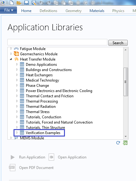
Verification models are available in the Application Libraries of COMSOL Multiphysics.
What if we want to verify our results in the absence of exact mathematical solutions and experimental data? We can turn to the method of manufactured solutions.
Implementing the Method of Manufactured Solutions
The goal of solving an IBVP is to find an explicit expression for the solution in terms of independent variables, usually space and time, given problem parameters such as material properties, boundary conditions, initial conditions, and source terms. Common forms of source terms include body forces such as gravity in structural mechanics and fluid flow problems, reaction terms in transport problems, and heat sources in thermal problems.
In the Method of Manufactured Solutions (MMS), we flip the script and start with an assumed explicit expression for the solution. Then, we substitute the solution to the differential equations and obtain a consistent set of source terms, initial conditions, and boundary conditions. This usually involves evaluating a number of derivatives. We will soon see how the symbolic algebra routines in COMSOL Multiphysics can help with this process. Similarly, we evaluate the assumed solution at time t = 0 and at the boundaries to obtain initial conditions and the boundary conditions.
Next comes the verification step. Given the source terms and auxiliary conditions just obtained, we use the simulation tool to obtain a numerical solution to the IBVP and compare it to the original assumed solution with which we started.
Let us illustrate the steps with a simple example.
Verifying 1D Heat Conduction
Consider a 1D heat conduction problem in a bar of length L
with initial condition
and fixed temperatures at the two ends given by
The coefficients A_c, \rho, C_p, and k stand for the cross-sectional area, mass density, heat capacity, and thermal conductivity, respectively. The heat source is given by Q.
Our goal is to verify the solution of this problem using the method of manufactured solutions.
First, we assume an explicit form for the solution. Let’s consider the temperature distribution
where \tau is a characteristic time, which for this example is an hour. We introduce a new variable u for the assumed temperature to distinguish it from the computed temperature T.
Next, we find the source term consistent with the assumed solution. We can hand calculate partial derivatives of the solution with respect to space and time and substitute them in the differential equation to obtain Q. Alternatively, since COMSOL Multiphysics is able to perform symbolic manipulations, we will use that feature instead of hand calculating the source term.
In the case of uniform material and cross-sectional properties, we can declare A_c, \rho, C_p, and k as parameters. The general heterogeneous case requires variables, as do time-dependent boundary conditions. Notice the use of the operator d(), one of the built-in differentiation operators in COMSOL Multiphysics, shown in the screenshot below.
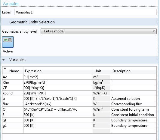
The symbolic algebra routine in COMSOL Multiphysics can automate the evaluation of partial derivatives.
We perform this symbolic manipulation with the caveat that we trust the symbolic algebra. Otherwise, any errors observed later could be from the symbolic manipulation and not the numerical solution. Of course, we can plot a hand-calculated expression for Q alongside the result of the symbolic manipulation shown above to verify the symbolic algebra routine.
Next, we compute the initial and boundary conditions. The initial condition is the assumed solution evaluated at t = 0.
The values of the temperature at the two ends of the bar are g_1(t) = g_2(t) = 500 K.
Next, we obtain the numerical solution of the problem using the source term, as well as the initial and boundary conditions we have just calculated. For this example, let us use the Heat Transfer in Solids physics interface.
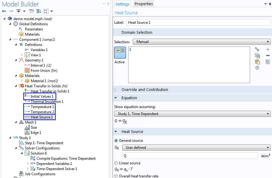
Add initial values, boundary conditions, and sources derived from the assumed solution.
For the final step, we compare the numerical solution with the assumed solution. The plots below show the temperature after a time period of one day. The first solution is obtained using linear elements, whereas the second solution is obtained using the quadratic elements. For this type of problem, COMSOL Multiphysics chooses quadratic elements by default.
")
")
The solution computed using the manufactured solution with linear elements (left) and quadratic elements (right).
Checking Different Parts of the Code
The MMS gives us the flexibility to check different parts of the code. In the example given above, for the purpose of simplicity we have intentionally left many parts of the IBVP unchecked. In practice, every item in the equation should be checked in the most general form. For example, to check if the code accurately handles nonuniform cross-sectional areas, we need to define a spatially variable area before deriving the source term. The same is true for other coefficients such as material properties.
A similar check should be made for all boundary and initial conditions. If, for example, we want to specify the flux on the left end instead of the temperature, we first evaluate the flux corresponding to the manufactured solution, i.e., -n\cdot(-A_ck \nabla u), where n is the outward unit normal. For the assumed solution in this example, the inward flux at the left end becomes \frac{A_ck}{L}\frac{t}{\tau}*1K.
In COMSOL Multiphysics, the default boundary condition for heat transfer in solids is thermal insulation. What if we want to verify the handling of thermal insulation on the left end? We would need to manufacture a new solution where the derivative vanishes on the left end. For example, we can use
Note that during verification, we are checking if the equations are being correctly solved. We are not concerned with whether the solution corresponds to physical situations.
Remember that once we manufacture a new solution, we have to recalculate the source term, initial conditions, and boundary conditions according to the assumed solution. Of course, when we use the symbolic manipulation tools in COMSOL Multiphysics, we are exempt from the tedium!
Convergence Rate
As shown in the graph above, the solutions obtained by the linear element and the quadratic element converged as the mesh size was reduced. This qualitative convergence gives us some confidence in the numerical solution. We can further scrutinize the numerical method by studying its rate of convergence, which will provide a quantitative check of the numerical procedure.
For example, for the stationary version of the problem, the standard finite element error estimate for error measured in the m-order Sobolev norm is
where u and u_h are the exact and finite element solutions, h is the maximum element size, p is the order of the approximation polynomials (shape functions). For m = 0, this gives the error estimate
where C is a mesh independent constant.
Returning to the method of manufactured solutions, this implies that the solution with linear element (p = 1) should show second-order convergence when the mesh is refined. If we plot the norm of the error with respect to mesh size on a log-log plot, the slope should asymptotically approach 2. If this does not happen, we will have to check the code or the accuracy and regularity of inputs such as material and geometric properties. As the figures below show, the numerical solution converges at the theoretically expected rate.
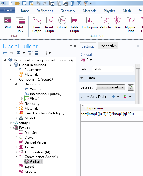
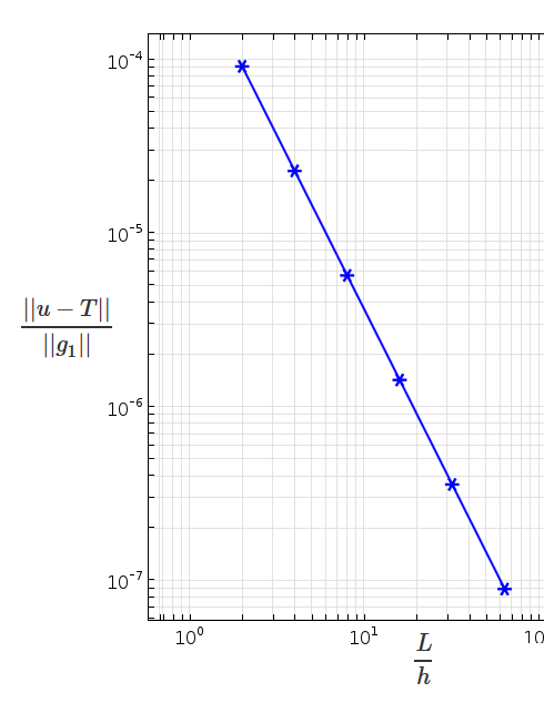
Left: Use integration operators to define norms. The operator intop1 is defined to integrate over the domain. Right: Log-log plot of error versus mesh size shows second-order convergence in the L_2-norm (m = 0) for linear elements, which is consistent with theoretical prediction.
While we should always check convergence, the theoretical convergence rate can only be checked for those problems like the one above where a priori error estimates are available. When you have such problems, remember that the method of manufactured solutions can help you verify if your code shows the correct asymptotic behavior.
Nonlinear Problems and Coupled Problems
In case of constitutive nonlinearity, the coefficients in the equation depend on the solution. In heat conduction, for example, thermal conductivity can depend on the temperature. In such cases, the coefficients need to be derived from the assumed solution.
Coupled (multiphysics) problems have more than one governing equation. Once solutions are assumed for all the fields involved, source terms have to be derived for each governing equation.
Uniqueness
Note that the logic behind the method of manufactured solutions holds only if the governing system of equations has a unique solution under the conditions (source term, boundary, and initial conditions) implied by the assumed solution. For example, in the stationary heat conduction problem, uniqueness proofs require positive thermal conductivity. While this is straightforward to check for in the case of isotropic uniform thermal conductivity, in the case of temperature dependent conductivity or anisotropy more thought should be given when manufacturing the solution to not violate such assumptions.
When using the method of manufactured solutions, the solution exists by construction. In addition, uniqueness proofs are available for a much larger class of problems than we have exact analytical solutions. Thus, the method gives us more room to work with than looking for exact solutions starting with source terms and initial and boundary conditions.
Try It Yourself
The built-in symbolic manipulation functionality of COMSOL Multiphysics makes it easy to implement the MMS for code verification as well as for educational purposes. While we do extensive testing of our codes, we welcome scrutiny on the part of our users. This blog post introduced a versatile tool that you can use to verify the various physics interfaces. You can also verify your own implementations when using equation-based modeling or the Physics Builder in COMSOL Multiphysics. If you have any questions about this technique, please feel free to contact us!
Resources
- For an extensive discussion of the method of manufactured solutions including relative strengths and limitations, see this report from Sandia National Laboratories. The report details a set of blind tests in which one author planted a series of code mistakes unbeknownst to the second author, who had to mine-sweep using the method described in this blog post.
- For a broader discussion on verification and validation in the context of scientific computing, check out
- W. J. Oberkampf and C. J. Roy, Verification and Validation in Scientific Computing, Cambridge University Press, 2010
- Standard error estimates for the finite element method are available in texts such as
- Thomas J. R. Hughes, The Finite Element Method: Linear Static and Dynamic Finite Element Analysis, Dover Publications, 2000
- B. Daya Reddy, Introductory Functional Analysis: With Applications to Boundary Value Problems and Finite Elements, Springer-Verlag, 1997
- Editor’s Note (1/16/20): The recently published COMSOL Verification and Validation Models page features dozens of models that demonstrate accurate solutions when compared against analytical results and established benchmark data. These models, which span all engineering fields, not only include reference values and sources for a wide range of problems but also provide step-by-step instructions to reproduce the expected results on your own computer. You are welcome to employ these models to further document your software quality assurance (SQA) and numerical code verification (NCV) efforts.


Comments (0)