Studies and Solver Updates
COMSOL Multiphysics® version 5.3 includes a new solver for CFD simulations and a new solver for electromagnetic and corrosion boundary element method simulations. Browse all of the COMSOL Multiphysics® version 5.3 updates relating to studies and solvers below.
Algebraic Multigrid (AMG) Solver for CFD
The smoothed aggregation algebraic multigrid (SA-AMG) method has been extended to work with the specialized smoothers for CFD in COMSOL Multiphysics®: SCGS, Vanka, and SOR Line.
Use of the alternative geometric multigrid (GMG) solver requires three mesh levels to be considered, which can create issues when trying to mesh and solve models with varying geometries of different sizes. The SA-AMG solver only requires one mesh level, making the meshing process much easier and the solving process much more robust for large problems and "difficult" geometries.
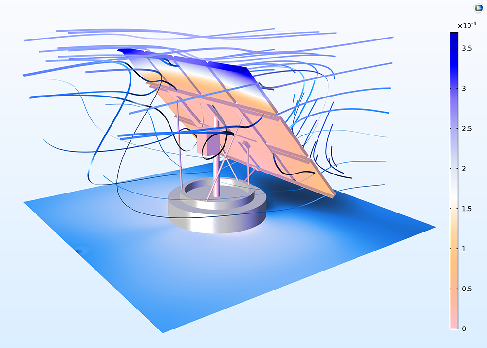
For example, in the fluid-structure interaction model of a solar panel (in the image), the struts and beams supporting the panels are small in comparison to the air domain surrounding it. This difference in dimensions makes it difficult to efficiently mesh the air domain together with the smaller parts and components, which would be made even more difficult if three meshes of different sizes are to be created. The SA-AMG solver requires only one mesh level, which is far easier to obtain.
Adaptation Integrated with Meshing Sequences and Error Estimation
The h-adaptation algorithm for stationary, parametric, and eigenvalue problems has been revised so that you can save the intermediate solutions and meshes. Furthermore, the resulting adapted meshes are now based on meshing features that make it possible to seamlessly switch from the automated solution process to manual adaptation when required.
To achieve this, two new meshing features have been introduced: Adapt and Size Expression. The Adapt feature refines your mesh based on either an expression for the error in your solution or by an expression for the desired mesh element size. Alternatively, the Size Expression node can be added to a meshing sequence in the Model Builder in order to vary element size throughout the modeling space using expressions. See the Mesh Updates page for more details.
The adaptation functionality and error estimation have also been unified such that the error estimates used by the adaptation method are now available as dependent variables to be used for postprocessing the results. Moreover, the L2-error (of the PDE residual) estimate is now also available for postprocessing.
Improvements have further led to the Mesh initialization method now being able to perform adaptation on meshes other than just the triangular and tetrahedral types. This is possible because adapted meshes are built with the Reference feature, which preserves the original mesh sequence together with the new Size Expression meshing feature.
The Regular refinement and Longest refinement methods now also automatically convert the mesh to triangles or tetrahedrons when needed. This means that there is no need for the user to add any Convert features to the meshing sequence.
 This Euler Bump benchmark model now uses the new adaptive mesh refinement functionality in COMSOL Multiphysics®.
Application Library path for an application using new adaptive mesh refinement:
CFD_Module/High_Mach_Number_Flow/euler_bump
Fast Iterative Solver for Boundary Element Method Problems
A dense direct solver is now available for solving problems best solved through the boundary element method (BEM). This is useful for applications not well suited for finite element method (FEM) modeling.
The solution time for this direct solver is approximately proportional to the cube of the number of degrees of freedom (DOF) in the problem. In other words, the solution time increases dramatically with problem size. To mitigate this, support is provided for iterative solvers based on fast matrix-vector multiplication. This enables matrices to be compressed using so-called ACA or ACA+ compression. These alternatives correspond to two different versions of the adaptive cross approximation method, which is a fast matrix multiplication method based on far-field approximations.
Two preconditioners are provided: the Sparse Approximate Inverse (SAI) and Direct Preconditioner. Both of these are exposed to the so-called near-field part of the matrix. The near-field part of the matrix is sparse and requires much less memory to store and solve for than the full matrix. The SAI preconditioner is an example of an explicit preconditioner that approximates the inverse of the matrix and not the matrix itself. The Direct Preconditioner uses the more common LU decomposition of the matrix.
BEM has been implemented in a general physics interface for solving PDEs, an interface for solving electrostatics applications in the AC/DC Module, and for solving electrochemical current density applications in the Corrosion Module and Electrodeposition Module.
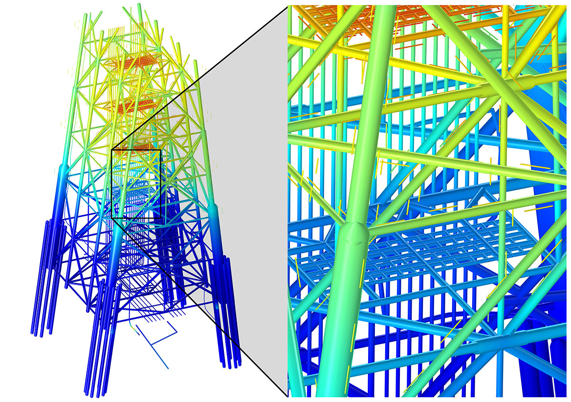 Modeling of the electrostatics properties of an oil rig in seawater using the boundary element method (BEM). The size, number of parts, and general complexity of the geometry, along with the unbounded region that the rig exists in, makes an example like this optimal for modeling with BEM. The overlay is a zoomed-in section of the oil rig that shows the finer details such as the sacrificial anodes, which are the thin rods next to the massive rig structure.
Application Library path for examples using BEM:
ACDC_Module/Capacitive_Devices/capacitor_tunable
ACDC_Module/Applications/touchscreen_simulator
ACDC_Module/Tutorials/capacitive_pressure_sensor_bem
Solver Support for Hybrid BEM/FEM Problems
Sometimes, multiphysics problems can be solved with one numerical method, but are optimally solved using different numerical methods — the boundary element method (BEM) and finite element method (FEM) — for the different physics. Hybrid BEM/FEM models can be used where the matrix storage is the optimal sparse format for the FEM part and a dense or matrix-free format for the BEM part. This makes it possible to use a separate preconditioner/smoother for the individual FEM and BEM parts of the matrix.
It is possible, for example, to use an efficient iterative solver with a hybrid preconditioner. The FEM part can rather freely be preconditioned as usual, while the BEM part can be used with one of the aforementioned preconditioners for the near-field matrix. The iterative method computes the residual with a hybrid matrix-based/matrix-free method, making optimal use of different sorts of fast matrix-vector products.
Sensitivity for Accurate Boundary Flux Variables
You can now obtain the sensitivity contribution from the Boundary Flux variables with the Forward sensitivity method. These are the accurate boundary flux variables that are available for some physics interfaces, such as mass and heat transfer. For these interfaces, select the Compute boundary fluxes check box under their respective Discretization sections to access and use these variables.
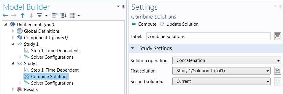
Combining Solutions
You can combine two solution objects into a single solution or data set. This is useful when one solution/data set is needed for postprocessing or when one solution is needed as an input for a new simulation. Time-dependent, parametric, and eigenfrequency solutions can be combined, and solutions can either be concatenated or summed.
Mesh-Based Performance Improvements in the Discontinuous Galerkin Method
Several improvements have been implemented to both speed up the discontinuous Galerkin (dG) method and to reduce its memory footprint. One improvement is a new mesh metric that is used for the calculation of the stable time step for the explicit time-stepping method that is used. This metric is the diameter of the largest inscribed circle for a triangle and largest inscribed sphere for a tetrahedron. This metric is better at determining what time step is needed in a stable fashion time-integrate and leads to a better characterization of the mesh elements at hand for a simulation.
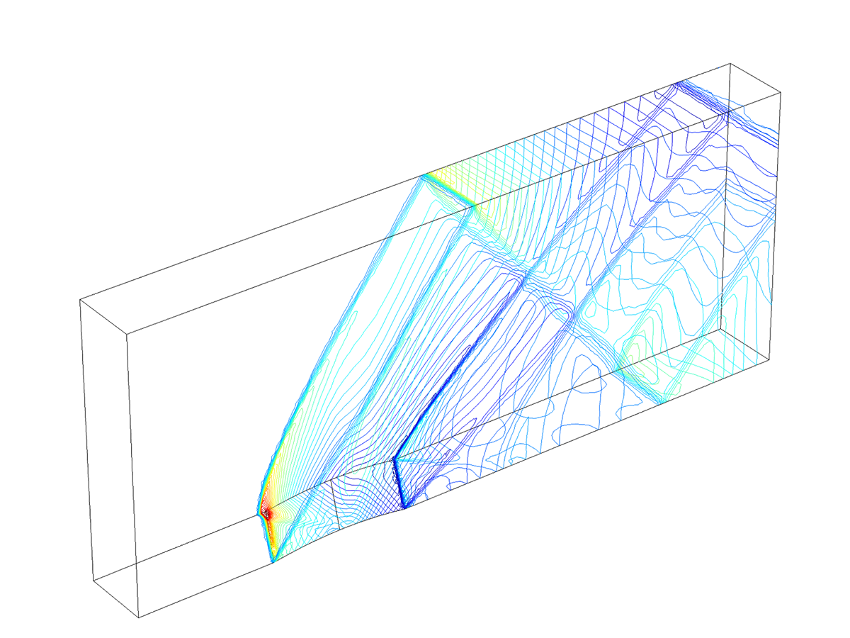
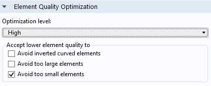
A second improvement has been achieved through a new mesh quality optimization procedure. This procedure should be used together with the dG method to further increase the stable time step for the explicit time-stepping method. This method changes the mesh to avoid cells that are too small and that would otherwise limit the stable time step. Use the new Avoid too small elements mesh option when generating a tetrahedral mesh in 3D (see image).
As an example, consider the Ultrasound Flow Meter with Generic Time-of-Flight Configuration tutorial model that contains 7.5 million degrees of freedom (DOF). In a test run on a desktop computer with an Intel Core™ i7 processor at 3.60 GHz with 4 cores and 32 GB of RAM, the acoustics problem is solved in 7 hours and 5 minutes and requires 6.0 GB of RAM in version 5.2a of COMSOL Multiphysics®. In version 5.3, with the new sparse assembly method, the same study solves in 5 hours and 1 minute and requires 5.8 GB of RAM. This represents a speedup of roughly 30% and a slight reduction in memory.
Multicore-Based Performance Improvements in the Discontinuous Galerkin Method
Reduction in memory has been achieved when running models on multicore systems. Here, a new sparse assembly method for the residual vector is used. The required memory is reduced and does not depend on the number of CPU cores that are used. Furthermore, the memory required during initialization has been substantially reduced. This improvement makes the method faster, since unnecessary allocation of memory is avoided.
In a further study of memory improvements when solving using multicores, separate from the improvements provided by the meshing and mesh metric parameters, we can compare a model solved in both COMSOL Multiphysics® version 5.2a and 5.3, where the exact same mesh and time step are used. Here, a simple wave equation simulation inside an ellipsoid using cubic basis functions is considered. The comparison is performed on an Intel® Xeon® CPU E5-1650 v4 at 3.60 GHz using 6 cores. Even without the mesh improvements, the CPU time reduction is around 18%. This memory reduction is expected to be even more pronounced when more cores are used.
| Size | Version 5.2a | Version 5.3 | Improvement |
|---|---|---|---|
| Medium (6.7 MDOF/t = 0.05) | 74 sec./4.1 GB | 61 sec./3.2 GB | 18%/22% |
| Large (20 MDOF/t = 0.05) | 307 sec./10 GB | 250 sec./7.3 GB | 19%/27% |
Intel, Intel Core, and Xeon are trademarks of Intel Corporation or its subsidiaries in the U.S. and/or other countries.