

Today, we will find out how to compute the total normal flux through a cross-section plane, passing through your simulation geometry. This can help us bridge the gap between simulations and experiments where, in the latter, it is often easier to physically measure the total flux. The approach discussed here works for any type of physics problem as long as we can identify the appropriate flux term corresponding to that physics.
What Is Flux?
Flux refers to the area density of any quantity that flows through a well-defined boundary of a domain. The domain could be a volume (in 3D), surface (in 2D), or edge (in 1D). Correspondingly, the boundary through which we compute the flux would be surface (in 3D), edge (in 2D), and point (in 1D), respectively. The total flux through the cross section is then the sum total of flux coming out of that boundary. Although this idea has its origin in the field of transport processes, the concept of flux and total flux can be related to many physics. This is because most physics are mathematically formulated based on some form of conservation equation. The following table provides a summary of flux-type physical quantities from different physics areas.
| Physics | Flux | Total Flux | ||
|---|---|---|---|---|
| Electrostatics | Electric displacement or Surface charge density (Unit: C/m2) | Surface charge (Unit: C) | ||
| Electric Currents | Current density (Unit: A/m2) | Current (Unit: A) | ||
| Magnetic Fields | Magnetic flux density (Unit: T) | Magnetic flux (Unit: Wb) | ||
| Mass Transport | Rate of Material flux (Unit: mol/m2s) | Material flow rate (Unit: mol/s) | ||
| Fluid Dynamics | Mass flux or Mass flow rate per unit area (Unit: kg/m2s) | Mass flow rate (Unit: kg/s) | ||
| Heat Transfer | Heat flux or Power per unit area (Unit: W/m2) | Power (Unit: W) | ||
| Structural Mechanics | Stress (Unit: Pa) | Force (Unit: N) | ||
Computing Flux
Now, let’s look at an example to find out the simple math behind computing flux.
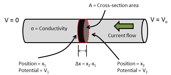
A simple example of computing current through a conductor.
Imagine a cylindrical conductor (shown above) through which electric current flows as a result of a potential difference across its two ends. Now, let’s focus on a small section of the conductor along its length (shown above as the red-dashed disk). The left and right ends of the disk are at position x1 and x2, respectively, and have a constant cross-section area of A. The electric potential on the left and right ends of the disk are V1 and V2, respectively. The electrical conductivity is denoted by σ. For electric current conduction, the flux physically signifies the total number of electrons flowing through the cross section per unit time (referred to as current density). Using Ohm’s Law, the current density (J) through this cross section can be computed from the following expression:
Now, in order to compute the current density through a cross-section boundary, let’s imagine that we squeeze the thickness of this disk, so that Δx ≈ 0. This helps us make the jump from algebra to differential calculus and express the flux through a boundary as:
Now, let’s make another jump from one-dimensional current conduction to a three-dimensional scenario where the electric potential as well as the conductivity could, in general, vary as a function of x-, y-, and z-coordinates. This would give us a current density vector:
Using notations from vector calculus, the above expression could be written in a more compact form:
Computing Total Normal Flux
Going back to our simple example, let’s say we are interested in finding out the total current passing through any arbitrary cross section of the conductor. For a straight cylinder with a constant cross-section area, we can easily find the total current passing through any section, by multiplying the cross-section area with the current density (flux).
What would you do for the three-dimensional case with the flux vector?
Here, we will follow the principles of integral calculus to find that out.
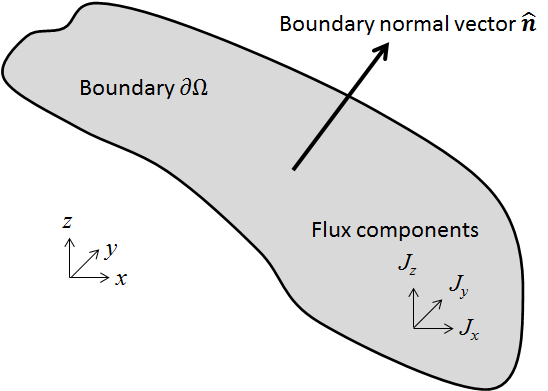
An arbitrary boundary (∂Ω) in 3D space whose normal vector is \hat{\bf n}=\begin{bmatrix} n_x & n_y & n_z\end{bmatrix}. The flux through this boundary is specified by the vector, \overrightarrow{\bf J}=\begin{bmatrix} J_x & J_y & J_z\end{bmatrix}.
To find the total normal flux through an arbitrary boundary, denoted by ∂Ω, we first need to find the normal flux through that boundary. This can be obtained from the dot product of the normal vector (\hat{\bf n}) of the boundary and the flux vector (\overrightarrow{\bf J}). The total normal flux can then be obtained by integrating this quantity over the boundary. The final expression used for computing the total normal flux would then be:
Computing Total Normal Flux in COMSOL Multiphysics
Now let’s find out how you can compute the total normal flux on a planar surface in the COMSOL software. We will look into two possibilities.
- When the planar surface is a 2D boundary (internal or external) of a 3D modeling geometry
- When the planar surface is not a part of the modeling geometry, but is created during postprocessing, using the Cut Plane data set feature
Model Overview
Let’s solve a DC electric current conduction problem on a bent copper wire whose two ends are at a potential difference of 1 mV.
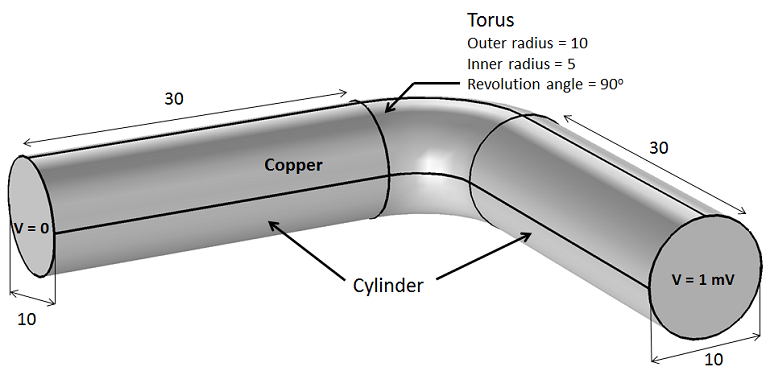
Overview of the electric current conduction model set-up. All geometric units are in millimeters (mm).
Here, we use the Electric Currents interface and a stationary study to solve a DC current conduction problem. A swept mesh is used on the geometry.
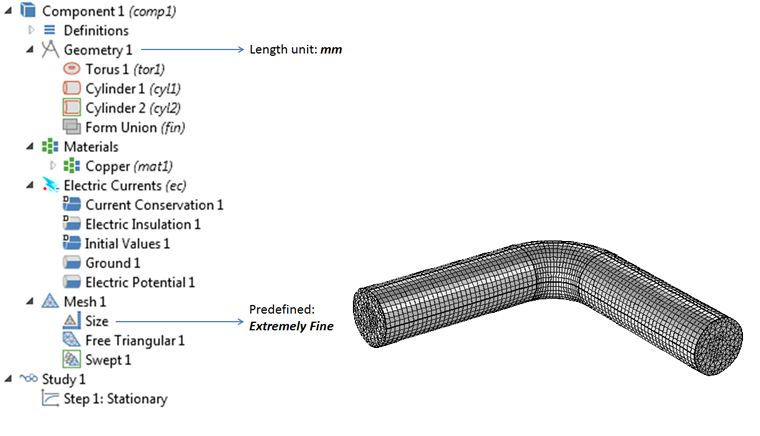
Representation of the problem in the COMSOL software.
Variation in Current Density
Before we proceed to compute the total current in the conductor, let’s take a look at the current density variation inside the conductor.
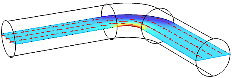
Spatial variation in the magnitude of current density and direction of current flow.
As moving charges try to take the shortest path (least resistance), we see that, in the curved section of the conductor, the current density varies through the volume significantly. It is largest near the inner radius and smallest near the outer radius.
Computing on a Geometric Boundary
Now, let’s turn our attention to one of the internal boundaries that connects the straight and curved regions.
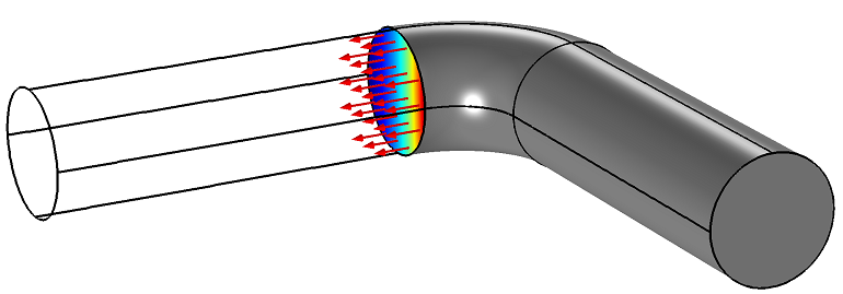
Spatial variation in the magnitude of current density on one of the internal geometric boundaries. The arrows show the direction of the normal vector of this boundary. Note that this direction coincides with that of the direction of the current flow.
In order to compute the total current flowing through this cross section, we will use the Surface Integration feature, which is available under Results > Derived Values.
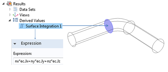
Snapshot of performing a surface integration to compute the area integral of the dot product of current density vector and surface normal vector.
Remember the integrand to obtain the normal flux: ( n_xJ_x+n_yJ_y+n_zJ_z ). For arbitrary geometrical shapes, this expression can be very complicated. The good news is that the COMSOL software contains automatic, built-in expressions for this, which can be used in both pre- and postprocessing. Here is how the expression looks in COMSOL Multiphysics:
nx*ec.Jx+ny*ec.Jy+nz*ec.Jz
Here, the components of the current density vector are available as built-in variables, namely, ec.Jx, ec.Jy, and ec.Jz. You can also find similar variables for the the flux quantity in other physics interfaces. The COMSOL software automatically computes the normal vector for all of the boundaries on the geometry. This information can be accessed by using the variables nx, ny, and nz.
Using this approach, we find the resulting current to be 62.9 A.
Computing on a Cut Plane
Now, let’s find out how you can implement the same idea on an arbitrary planar surface that cuts through the modeling geometry.
Creating a Cut Plane
You can use the Cut Plane feature under Results > Data Sets to create such a planar surface. There is no need to go back and change the actual modeling geometry to insert this surface and solve the model again. This is a big advantage when you decide to visualize or compute some quantity on an arbitrary planar surface. The cut plane can be created using two alternate approaches.
- Add one under Results > Data Sets
- This gives you a default set of coordinates for three points that define the cut plane
- You can then manually modify the coordinates to get the desired plane
- Click on an existing plot group and use some of the buttons on the ribbon
- This gives you the added flexibility to drag a slider bar and move the plane around
- COMSOL Multiphysics also automatically creates a Cut Plane branch (under Results > Data Sets) with information on the coordinates of the three points in space that defines this plane
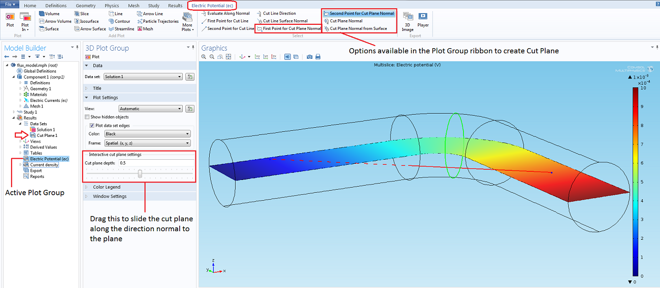
Screenshot showing the options to create a cut plane. The green line in the Graphics window represents the boundary of the cut plane intersecting the modeling geometry. The red line is the normal of the cut plane. (Click to enlarge)
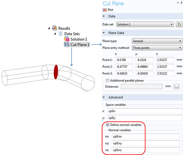
Screenshot of the Settings window for the Cut Plane branch, which is found under Results > Data Sets. Variable names for the surface normal vector can be invoked from the Advanced settings, by checking the “Define normal variables” checkbox.
Surface Normal of a Cut Plane
In order to access the variables corresponding to the normal vector of the cut plane, you would need to look under the Advanced section in the settings window of the Cut Plane data set branch and check the box to “Define normal variables“. This will invoke the variables cpl1nx, cpl1ny, and cpl1nz. The default naming convention for these variables uses the tag name (cpl1) attached to the Cut Plane 1 data set. So, if you create another cut plane, its normal variables will automatically be given a different name. You can also replace these default variables names with other names of your choice.
The COMSOL software computes the cut plane normal vector from the cross product of the two base vectors that define the plane. These base vectors are computed from the coordinates of the three points that are used to define the cut plane.
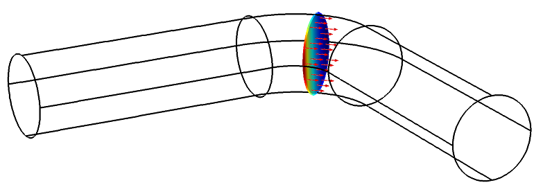
Surface plot of the magnitude of current density on the cut plane and an arrow surface plot showing the cut plane normal vector with red arrows.
Computing the Surface Integral
Finally, let’s find out how we can compute the total normal flux (current) passing through the cut plane.
Once again, we use the Surface Integration feature. This time, we need to ensure that the data set for the Surface Integration branch is set to Cut Plane 1 (or the desired cut plane data set, if you have multiple cut planes).
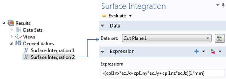
Snapshot of performing a surface integration to compute the area integral of the dot product of current density vector and surface normal vector of the cut plane.
The expression that we integrate over the surface of the cut plane is the following.
-(cpl1nx*ec.Jx+cpl1ny*ec.Jy+cpl1nz*ec.Jz)[1/mm]
Here, the negative sign that precedes the expression is used, because the direction of the cut plane normal is opposite to that of the direction of current flow. Also, note the normalization of the unit by using the [1/mm] factor. This is done to take into account the fact that the modeling geometry uses the millimeter as the length unit of choice. Using this approach, once again, we confirm the resulting current to be 62.9 A.
Now you just need to open your favorite COMSOL Multiphysics model and try out what you learned here on any other physics of your choice.
Further Reading
You can learn more about postprocessing in COMSOL Multiphysics from the videos and blogs available on our website.


Comments (9)
Lingling Tang
June 9, 2014Why the surface integration of variable “ec.normJ” is a little bigger than that the integration of expression “nx*ec.Jx+ny*ec.Jy+nz*ec.Jz”?
and, secondly, the negative sign in “-(cpl1nx*ec.Jx+cpl1ny*ec.Jy+cpl1nz*ec.Jz)[1/mm]” is not necessary if the order of selecting the “first point for cut plane normal” and the second point is changed.
Supratik Datta
June 9, 2014Hi Lingling, Thanks for taking out the time to read this blog. Let me address your questions.
1. The variable ec.normJ is the L2 norm of the current density vector. This is usually not the same as the normal component of the same vector on a given surface. In the Electric Currents interface COMSOL actually stores the normal current density in another variable which is ec.nJ. So you can actually replace “nx*ec.Jx+ny*ec.Jy+nz*ec.Jz” with “ec.nJ” and try out again.
2. You are right about the negative sign. The only purpose of showing it in this blog is to highlight that in case you have created the cut plane in such a way that its normal vector points in exactly the direction, that is opposite of what you want, instead of trying to create another cut plane, you can simply type in the negative of the normal vector variables to obtain the desired direction.
Oscar Diaz
April 23, 2015Dear Supratik,
I’m trying to evaluate electric charge in a certain potential arrangement. My main domain is a big cylinder, where the bottom plane is ground, the other faces are zero charge/continuity and inside there are two sphere ‘electrodes’ where I can fix an electric potential. If I enclose these electrodes in a single gaussian surface, the value of the surface integral of es.normD changes with the size of the enclosing gaussian surface…
I’ve tried modifying the mesh size, using electric potential or surface charge on the electrodes, using an infinite element domain on the external wall of my main domain, but still the result I get from the integral changes with the size of the enclosing surface. Do you have any suggestions? How can I send you a file with the model so you can take a look?
Thanks
Supratik Datta
April 23, 2015Hello Oscar,
Please see the following tutorial.
http://www.comsol.com/model/computing-the-effect-of-fringing-fields-on-capacitance-12605
Also, feel free to contact our technical support team.
http://www.comsol.com/support
Syed Tauseef Hossain
July 5, 2016Dear Supratik,
I am assuming a similar method can be applied to determine the normal stress at a boundary
similar to what shown here. I can get the stress vector i.e. S=sigma.n, where sigma the stress tensor and n is the unit vector normal to the plane. Then, sigma_N=S.n to determine normal stress along the normal direction to that boundary.
But, what about the shear stresses? Presumably the same method can be applied i.e. tau=S.t1 (in comsol!?) and tau=S.t2. But these are well suited for the cartesian coordinate. However, I am having difficulty for a circular boundary like the one shown above to get the two shear stresses, especially when the model contains both circular and rectangular objects. As a result I am unable to use a cylindrical coordinate system. Can you please help on this?
Ali Mehrabifard
February 3, 2017Thank you for your great help, by this simple examples. There is a fact that this technique cannot accurately compute the variables of my interest. In other words, I built two cylindrical wellbores, one of which is injection and the other one is production in a porous media. I sat a value of Qm for the mass flux injection on the injection wellbore, however when I am computing such a value on injection wellbore surface by this technique the value is far different. I googled this problem and many researchers faced same problem, I found some ways one was remeshing but this technique needs more RAM memory (I am using 32 GB RAM memory), which is not available now. on the other hand, there is another way by weak constraint but in this regard I am not sure if I could fully follow the instruction and there is always an error which says that some equations are empty in some coordinates. As I understood, Lagrangian Multiplier method is being used to find the minimum or maximum of an objective function on a constraint function and special boundary condition, so I just confused, how we can use Weak Constraint to impose a variable on a surface by Lagrangian Multiplier?
Thanks in advance,
Ali
Ali Mehrabifard
February 3, 2017Thank you for your practical note. I am using this technique to compute the mass flux in my doublet system in which there are two cylindrical shape wellbores, one of which is injection and the other one is production in a porous media. I sat a constant injection rate for the injection wellbore, and I interested in calculating the production rate on the production wellbore. However, in such a calculation, there is a point that when I am calculating the mass flux for injection well it is far different from the imposed value which I already sat. Accordingly, the other calculation including production mass flux (rate) is not reliable and indeed logically they are far from the expected values. I found some solutions, since it was the problem that many users are being faced. One solution was to remesh the model, I did that for a simple 2D it was working, but for the 3D model, the RAM memory is not supporting the calculations (I am using a 32 GB RAM memory). The other solution is to impose the injection flux (rate) by Weak Constraint, in this sense, based on my best knowledge, Lagrangian Multiplier method which is using here is a method by which maximum and minimum of an objective function is being calculated when there is a constraint function and boundary conditions. I got confused, how Weak Constraint can help me out?
Chunlou Li
April 4, 2017Supratik, thanks a lot for the posting! my question is how to assign a total flux (integral) as a boundary condition? Appreciated.
Ruud Borger, COMSOL employee
April 18, 2017Hi Chunlou,
It depends on the physics area, but usually we have a built-in option for the total flux. For instance, in “Heat flux”, you can specify Heat rate (W). In Electric Currents, you can use a Terminal to specify the total current (A), and in Solid Mechanics, you can add a Boundary Load as Total force (N).
You can also add a global equation (ODE) to specify the total flux (integral).
I hope that helps.