

Solution methods are a valuable tool for ensuring the efficiency of a design as well as reducing the overall number of prototypes that are needed. In today’s blog post, we introduce you to a particular type of method known as multigrid methods and explore the ideas behind their use in COMSOL Multiphysics.
An Overview of Solution Methods
The differential equations that describe a real application admit an analytical solution only when several simplifying assumptions are made. While the insights we gain from this approach are valuable, they are not enough to confirm that our design is efficient or to reduce the number of prototypes that are needed to obtain a complete understanding.
Numerical solution methods for models based on partial differential equations (PDEs) associated with your engineering problem overcome such limitations and allow you to represent the problem as a system of algebraic equations. Linear algebraic problems in matrix form as Au = f, where u is the vector solution, are often a central part of the computational problem for the numerical solution process. Once we have determined A and f, all we have to do is to “find” u.
When it comes to solution methods for linear algebraic problems, they can either be direct or iterative. Direct methods find an approximation of the solution A^{-1}f=u by matrix factorization in a number of operations that depend on the number of unknowns. Factorization is expensive, but once it has been computed, it is relatively inexpensive to solve for new right-hand sides f. The approximate solution u will only be available when all operations required by the factorization algorithm are executed.
Iterative methods begin with an approximated initial guess and then proceed to improve it by a succession of iterations. This means that, in contrast to direct methods, we can stop the iterative algorithm at any iteration and have access to the approximate solution u. Stopping the iterative process too early will result in an approximate solution with poor accuracy.
Direct or Iterative?
When it comes to choosing between direct or iterative solution methods, there are several factors to consider.
The first consideration is the application and the computer that is used. Since direct methods are expensive in terms of memory and time intensive for CPUs, they are preferable for small- to medium-sized 2D and 3D applications. Conversely, iterative methods have a lower memory consumption and, for large 3D applications, they outperform direct methods. Further, it is important to note that iterative methods are more difficult to tune and more challenging to get working for matrices arising from multiphysics problems.
As you can see, many different variables come into play when we have to make a decision about the best solver for the problem at hand. My suggestion is to use a simulation software that allows you to access the best-in-class solution methods. This means that you will be able to tackle your application with the right tools since your choice will be based on the physics involved and the computational resources that are available. It is indeed a good time to simulate your application since solution methods have improved at a rate even greater than the hardware, which has exploded in capability within the past several decades (see the plot below). All of the solution methods mentioned in the plot are available in COMSOL Multiphysics.
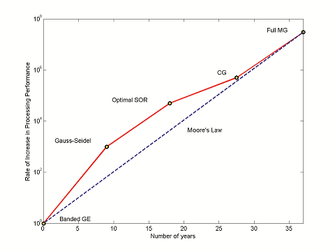
A plot highlighting the increasing performance rate of solution methods (solid) and hardware (dashed) as compared to time. Legend: Banded GE (Gaussian Elimination, direct method), Gauss-Seidel (iterative method), Optimal SOR (Successive Over Relaxation, iterative method), CG (Conjugate Gradient, iterative method), Full MG (Multigrid, iterative method). Source: Report to the President of the United States titled “Computational Science: Ensuring America’s Competitiveness”, written by the President’s Information Technology Advisory Committee in 2005.
My colleagues developing the solvers in COMSOL Multiphysics continually take advantage of these improvements, ensuring that we offer you high-performance methods. The rest of this blog post will focus on discussing the main ideas behind multigrid methods, as they are the most powerful of methods.
Why Multigrid Methods Are Necessary
In order to introduce you to the basic ideas behind this solution method, I will present you with numerical experiments exposing the intrinsic limitations of iterative methods that multigrid methods are built on. For the sake of brevity, I will analyze only their qualitative behavior (I suggest you read A Multigrid Tutorial by William L. Briggs for more details on what is mentioned here).
Let’s start iterating with an approximated initial guess consisting of Fourier modes. They can be written as \sin (x · \cdot k · \cdot \pi), where k is the wave number and 0 \leq x \leq 1.
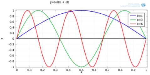
Fourier modes with k = 1,3,6. The kth mode consists of k half sine waves on the domain. For small values of k, there are long smooth waves. For larger values, there are short oscillatory waves.
The qualitative plot below shows that convergence is slower for smooth waves and quicker for oscillatory waves. Smooth waves are detrimental for the performance of these simple iterative methods — an intrinsic limitation. Typically, an approximated initial guess will contain several Fourier modes and convergence will start to slow down after the first iterations. This is because oscillatory components are efficiently eliminated from the error, while the smooth ones prevail and are left almost unchanged at every iteration. In other words, convergence is stalling. This is the reason why simple iterative methods don’t perform well. They converge too slowly for small wave numbers.
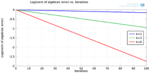
Log of the maximum norm of the algebraic error plotted against the iteration number for three different initial guesses (k = 1,3,6).
It is possible to overcome the limitations of simple iterative methods by modifying them to increase their efficiency for all Fourier modes. Let’s take a look at how multigrid methods take advantage of such limitations.
Say, for instance, that we also use a coarse grid during the solution process. There are a few good reasons to do this…
To start, the error associated with smooth waves will appear to have a relatively higher wave number, meaning that convergence will be more effective. Secondly, it’s cheaper to compute an improved initial guess for the original grid on a coarse grid through a nested iteration procedure. Clearly, restriction and prolongation methods need to be developed for mapping from one grid to another. Lastly, the residual correction procedure can also benefit from treatment on a coarse grid when convergence begins to stall, leading to the idea of coarse grid correction.
We’ll share more details about nested iteration and coarse grid correction in a follow-up blog post. Stay tuned!
Further Reading
Editor’s note: This blog post was updated on 4/15/16.

Comments (0)