

We can leverage simulation software to understand and optimize component design. Every simulation relies on a model that is a representation of the reality that the application finds itself in. Modeling enables us to represent this reality with enough detail to receive relevant information about the particular application or component. Let’s have a look at a thermal stress analysis of the turbine stator blade model from our Model Gallery and investigate the effects of heat transfer and thermal stress that are so important in this application.
Efficient Heat Transfer Modeling
For fast computation, the heat transfer aspect of the turbine stator blade model can be predefined, and not specifically solved for. Note that the modeling level shown here can be the final goal of a study, or it can be used as the first step in receiving an overview of the model and verifying that all the settings are consistent. Regardless of which case pertains to you, I always recommend starting with a version of a model where it is easy to verify the behavior with different parameter sets. It is also invariably better if the model does not require hours or days to return a result. (Such computations should be run only after the validation of initial versions of the model as the final simulation before manufacturing or for reasons of quality assurance.)

Stator blade geometry with mounting details, the blade between them, and a cooling duct within the blade.
Modeling Thermal Stress in a Turbine Stator Blade
Let’s use the Thermal Stress Analysis of a Turbine Stator Blade model as an example of how an efficient model can remain accurate by defining several modeling details. The stator consists of a duct within the blade that is used to pass a fluid through the stator in order to cool the structure. Heat is also passed between the surroundings and the stator’s surfaces at a significant rate, due to the fact that the stator blade is subjected to high velocities.
The key to accelerating the computation of the model is to use average Nusselt number correlations — instead of simulating complicated flow in the duct and around the blade — to estimate a heat transfer coefficient between the fluids and the structure. With some experience or a literature review, you can find average Nusselt number correlations that provide a decent representation of the heat exchange process.
Predefined and User-Defined Expressions
In the stator blade model, some of the heat exchange coefficients are established using classical conditions, while some parts of the model do not fit in any classical configuration. Instead, these parts require tailored formulations that have been validated for analog situations. For the classical conditions, the Heat Transfer Module equips you with predefined correlations. For the parts that need tailored formulations, you are able to enter the particular expression you need right into the software.
Setting up the Model
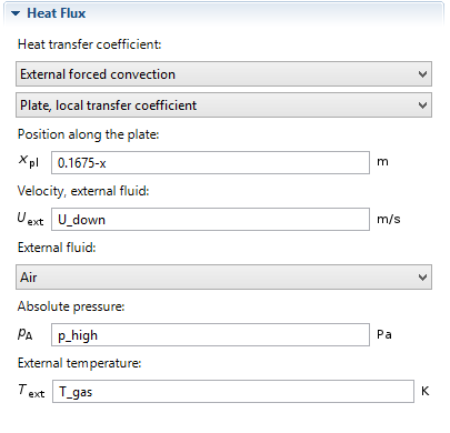
The pressure side (the concave front of the blade) and the suction side (behind the blade) are approximated as two flat plates using the local heat transfer coefficient for external forced convection. These Nusselt correlations are predefined and can be selected from a list. The interface then provides inputs for the quantities needed to define the correlation: the nature of the fluid, its state (temperature and pressure), and its velocity. The combustion gases are approximated as air at 30 bar and 1,100 K. The corresponding speed of sound is approximately 650 m/s. A typical Mach number is 0.7 on the pressure side, and 0.45 on the suction side. This corresponds to approximately 450 m/s (called U_up in the model) on the pressure side, and 300 m/s (called U_down in the model) on the suction side. For more accuracy, we use a local transfer coefficient rather than an averaged coefficient. Therefore, in addition to former quantities, this requires the position along the boundary that is defined using the global coordinate system.
The figure below shows all these settings entered into the predefined physics interface:
The mounting walls adjacent to the stator blades are treated in the same way as the stator itself, but with the free stream velocity set to 350 m/s.
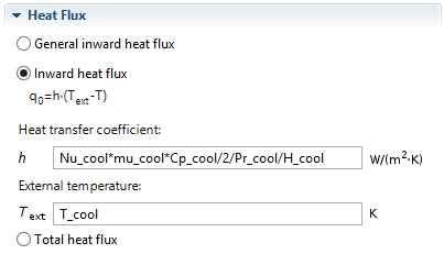
The blade also exchanges heat with the air flowing through the cooling duct, shown below. The duct geometry is simplified and does not include details, such as the ribs that are used to increase the cooling surface area. With this representation, we can calculate an equivalent heat transfer coefficient with the help of the average Nusselt number correlation from J. Bredberg’s thesis “Turbulence Modelling for Internal Cooling of Gas-Turbine Blades“. In this case, the cooling temperature is T_cool = 800 K.

The blade’s internal cooling duct.
Because this correlation is quite original, it is not predefined in the software. This is not an issue of course, since it is possible to enter any user-defined expressions directly into the model settings window. In fact, any algebraic expression can be entered into COMSOL just as easily as it can be written on a piece of paper. Here, you can see how the heat transfer coefficient has been defined by combining different parameters in the figure below:
In the blade itself, heat transfer by conduction is defined to be the operating physics. The blade is assumed to be made of the M-152 alloy, which is a 12% chromium steel alloy with high tensile strength (see M.P. Boyce’s Gas Turbine Engineering Handbook). Note that the structural and other material properties of the M-152 alloy are available in COMSOL’s Material Library.
Thermal and Stress Analysis Results
The turbine stator model contains the heat transfer model described above, coupled with a structural mechanics analysis to return the thermal stress. Earlier, I defined modeling as representing reality with a correct level of detail in order to obtain the relevant information about the application. So what information did we obtain here?
The thermal analysis primarily accounts for the flow parameters, which can be investigated in detail. Looking at the temperature profile in the image below, we can see that the trailing edge reaches a temperature close to that of the combustion gases. This indicates that the imposed cooling through the duct might be insufficient, either due to the forced rate of cooling fluid, the fluid temperature, or the actual design of the cooling.

Temperature field on the blade surface.
For the stress analysis, the results show two interesting things. The first is regarding the blade’s design: the imported geometry contains sharp angles, which are known to result in high levels of stress in their immediate surroundings. This means that the geometry should be reworked to be rid of these artifacts, as the manufactured stator blade would almost certainly not contain them. Yet, despite this, the structural analysis still shows that the maximum displacement is about 2 mm, which is an acceptable operating condition.

Displacement magnitude and deformation (amplified 10 times) of the blade.
Second, the maximum stresses are located around the region of the cooling duct where the thermal differentials are highest. This indicates that the cooling process has to be carefully designed and can’t be arbitrarily increased by decreasing the cooling temperature without running the risk of structural damage. It also indicates that, for this working regime, the thermal design may not neglect film cooling.
Further Resources
- Model Download: Thermal Stress Analysis of a Turbine Stator Blade
- Previous blog post: Turbine Stator Blade Cooling and Aircraft Engines


Comments (0)