

If you use finite element simulation software, such as COMSOL Multiphysics, you will come across the expression “weak form” at some point. When you do, you may wonder what this expression means. Weak form is actually a very powerful concept. Here, you will learn about its basic ideas and corresponding benefits.
The Origin of Weak Equations
Multiphysics simulations are based on partial differential equations (PDEs). These PDEs are typically derived from conservation laws of physical principles, such as conservation of mass, energy, and momentum. These well-known conservation laws can, without any further assumptions, be formulated as integral equations over arbitrary domains.
Volume integral terms describe what is stored inside the domains or added by sources, while surface integrals describe the interaction with neighboring domains or an external environment. Provided that all involved functions are smooth enough, the divergence theorem by Gauss can transform the surface integrals into volume integrals. Since the domain used in the derivation is arbitrary, the resulting equation must be valid at every point individually, turning the integral equation into a PDE.
There is, however, a slight flaw in this standard PDE derivation procedure: the functions involved (material properties, in particular) are not always smooth enough to justify the application of Gauss’s law everywhere. The resulting PDE is, therefore, too strict in the sense that it does not allow all physically sensible solutions (this is where the weak form comes into play). The weak equation partially reverses the derivation procedure to return an integral formulation, which is less strict than the PDE. This means that weak equations are actually closer to the underlying physics than classic equations.
How to Derive a Weak Equation from a Classic Equation
We will begin with the PDE and outline the typical procedure for deriving its weak counterpart. To this end, let’s consider the diffusion equation:
Most of the equations in the COMSOL software involve similar terms. For heat transfer applications, the diffusion coefficient, c, and the source term, f, refer to the thermal conductivity and a heat source, respectively. If the unknown function, u, is a solution of the original PDE, it is also a solution of the following integral equation:
This results from multiplying the PDE with an arbitrary function, v, followed by applying the integral over \Omega on both sides of the equation.
Conversely, a function, u, that solves the integral equation for a sufficient number of different functions, v, is a likely candidate for solving the original PDE. That is why the functions, v, are called test functions and play a key role in the finite element method. We will discuss the choice of test functions in the section below.
The transformation of the PDE into this integral equation already reflects the nature of the weak form, but is usually followed by a second step. This step applies the divergence theorem by Gauss or Green’s formula (also known as integration by parts) on second order derivatives. In our example, we can rewrite the left-hand side of the previous integral equation as:
with \partial \Omega being the boundary of the domain, \Omega, and n the normal vector oriented away from the domain. Using this formula, the final weak form of the diffusion equation reads:
The boundary integral is responsible for the interaction with the surrounding of \Omega. Here, boundary conditions come into play, which describe this interaction and, thereby, make the whole problem unique. When we simulate heat transfer, the term -c\nabla u\cdot n describes the heat flux over the boundary, for example. If there is no heat flux, the boundary is thermally insulated.
The Choice of Test Functions
A function, u, is called a weak solution of the PDE if it solves the weak equation for many different test functions, v. More precisely, we not only consider one test function, but v represents a whole class of test functions where each one corresponds to an equation. Of course, we could never consider all possible test functions as this would result in an infinite amount of equations. In practice, we need a finite number of well-chosen test functions. This is where finite elements come into play.
You all know that the computational domain needs to be meshed before running your study. Meshing divides the geometry into a set of smaller volumes — elements. Test functions can then be defined using polynomials on each element such that they are non-zero only on a small group of neighboring elements, and zero outside the group. The most common type of polynomials, constructed in this way, are known as Lagrange shape functions and are used by the COMSOL software for many physics interfaces.
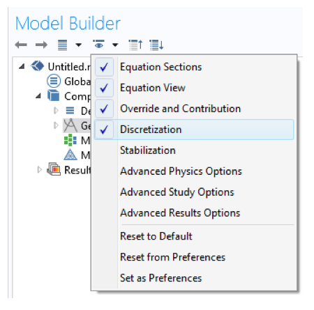
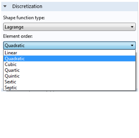
Selecting Discretization (left). In the Discretization settings, Lagrange elements are used by default (right).
There are also other possible test functions exist, but we won’t discuss those details here. The important thing to note is that since test functions associated with different mesh elements are independent, the mesh effectively decides the number of test functions, as well as their spatial resolution.
What does all this have to do with your solution? The resulting solution of your computation is actually a superposition of all involved test functions. The message here is that although your true solution might be a rather complex function, it can be approximated as a combination of very simple functions. The finer the mesh, the more shape functions are involved and the better the solution will be (especially in regions with steep gradients, as more mesh elements are needed). If you keep refining the mesh until your solution does not change anymore, you have successfully performed a mesh convergence study and your solution is likely to be a good approximation of the original PDE’s solution.
This method of using the test functions to approximate the solution is called the Ritz-Galerkin approach and is, in some sense, the best finite element approach as it minimizes the error of the calculated and exact solution. There is a lot more to cover on the topic of discretization, such as meshing and convergence. For now we’ll add the following plot, which could represent a bending membrane under a given load. It shows piecewise linear approximations of the solution with an increasing mesh resolution.

Example of how a solution improves for an increasing number of linear shape functions.
What Happens in the Mathematical Limit?
Theoretically, the mesh resolution can be increased further, meaning that the set of test functions becomes larger. You can imagine that the mathematical limit of this procedure results in a set of test functions, which is, in some sense, complete and continuous. This is not relevant from a practical point of view, but the argument leads towards a sound mathematical theory of solvability and uniqueness of solutions. Although you, as a COMSOL Multiphysics user, do not need to deal with these issues, it will be comforting to know that there is a sound theoretical basis of your calculations.
The Weak Equation in COMSOL Syntax
At this point, you may be wondering how the weak form is expressed in COMSOL syntax. To this end, the software provides the test operator, which is used to express the test functions, v. The test operator operates on the solution variable, u, and its derivatives, i.e., v=\mathrm{test}(u). There is a logical reason for associating test functions with the solution in this way. If the solution is represented using a polynomial basis on the mesh, as described above, using the same basis for the test functions ensures that the discrete system contains the same number of unknowns and equations.
In order to translate the first term of the weak equation of our example into COMSOL syntax, we first need to rewrite the gradients by means of the partial derivatives with respect to x, y, and z. Here, the notation for the first partial derivative is \frac{\partial u}{\partial x}=ux.
Similarly, partial derivatives of the test function are expressed as \frac{\partial v}{\partial x}=\mathrm{test}(ux).
Altogether, the domain integral terms of the weak form read in COMSOL syntax as:
The boundary terms require special treatment, which is beyond the scope of this blog post. No equals sign needs to be included, since the weak form PDE is automatically set to zero. It is important to note that this translation is normally done automatically because COMSOL Multiphysics needs the weak form to proceed with the calculation. However, it is also possible to enter a weak form as a user. The default domain Weak Form PDE interface suggests the above equation with c=f=1 and a change of sign, as shown in the following screenshots:
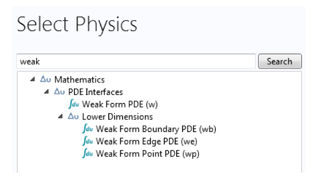
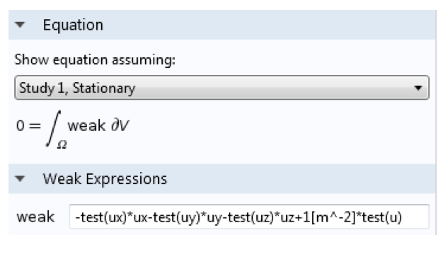
Weak form interfaces available in COMSOL Multiphysics (left). Example of how to enter the weak form in COMSOL syntax (right).
Benefits of the Weak Form Approach
What does all of this mean in practice? The real world is not always nice and smooth. It can show kinks in material data, rough surfaces, point sources, or rapid changes in the solution or its gradient. While classic PDEs reach their limits for non-smooth physical effects, weak equations are most often very suitable. They are less strict because all involved terms are integrals over mesh elements and don’t need to be well-defined at every single point in the domain. This is the key benefit of the finite element approach, which enables the COMSOL software, and you, as a user, to get solutions for your real-world applications.
To sum up, weak equations:
- Are sets of integral equations. The mesh dictates the number of equations solved in your study.
- Allow for real-world modeling because they directly emerge from the underlying physical conservation law.
- Come along with a sound mathematical theory of solvability and uniqueness of solutions.

Comments (9)
Nagi Elabbasi
May 5, 2014That was, in my opinion, a very good description of the weak form, its theoretical framework, and its benefits, with just the right amount of mathematics.
Yaohui Chen
May 14, 2014Much better than the old manual I searched three years ago.
Amin Parvizi
July 30, 2014I really enjoyed reading this post…Thanks.
Peter Cendula
November 12, 2014Thanks good article. Are you planning to do similar post for boundary conditions in weak form, that would be useful for us!
Andrew Griesmer
November 19, 2014Hi Peter, we actually just posted a similar blog post today that discusses boundary conditions. Hope it’s what you’re looking for!
http://www.comsol.com/blogs/brief-introduction-weak-form
Malkhaz Meladze
November 20, 2014A very clear exposition. Thank you.
Camille S.
February 11, 2015Hello Peter,
Thanks you for this great explanation.
I am using the weak form PDE with 2 dependant variables on Comsol 5.0, and I do require two weak expressions (otherwise I get the message : “invalid parameter value : weak expressions cannot be empty”) I am not sure of the second expression I have to use. Do you have any idea ?
Thanks a lot
Neo Shvr
February 15, 2015Good Article.
If you can also add some references for advance study, that will be great.
Thanks
Bettina Schieche
February 18, 2015Hallo Neo Shvr,
any textbook on Finite Elements can be used for advance study. Some more details on weak forms in COMSOL can be found in the following blog posts:
http://www.comsol.de/blogs/brief-introduction-weak-form/
http://www.comsol.de/blogs/discretizing-the-weak-form-equations/
http://www.comsol.de/blogs/implementing-the-weak-form-in-comsol-multiphysics/
Bettina