

In structural mechanics you will come across a plethora of stress and strain definitions. It may be a Second Piola-Kirchhoff Stress or a Logarithmic Strain. In this blog post we will investigate these quantities, discuss why there is a need for so many variations of stresses and strains, and illuminate the consequences for you as a finite element analyst. The defining tensor expressions and transformations can be found in many textbooks, as well as through some web links at the end of this blog post, so they will not be given in detail here.
The Tensile Test
When evaluating the mechanical data of a material, it is common to perform a uniaxial tension test. What is actually measured is a force versus displacement curve, but in order to make these results independent of specimen size, the results are usually presented as stress versus strain. If the deformations are large enough, one question then is: do you compute the stress based on the original cross-sectional area of the specimen, or based on the current area? The answer is that both definitions are used, and are called Nominal stress and True stress, respectively.
A second, and not so obvious, question is how to measure the relative elongation, i.e. the strain. The engineering strain is defined as the ratio between the elongation and the original length, \epsilon_{eng} = \frac{L-L_0}{L_0}. For larger stretches, however, it is more common to use either the stretch \lambda=\frac{L}{L_0} or the true strain (logarithmic strain) \epsilon_{true} = \log\frac{L}{L_0} = \log \lambda.
The true strain is more common in metal testing, since it is a quantity suitable for many plasticity models. For materials with a very large possible elongation, like rubber, the stretch is a more common parameter. Note that for the undeformed material, the stretch is \lambda=1.
In order to make use of the measured data in an analysis, you must make sure of the following two things:
- How the stress and strain are defined in the test
- In what form your analysis software expects it for a specific material model
The transformation of the uniaxial data is not difficult, but it must not be forgotten.
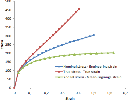
Stress-strain curves for the same tensile test.
Geometric Nonlinearity
Most structural mechanics problems can be analyzed under the assumption that the deformations are so small compared to the dimensions of the structure, that the equations of equilibrium can be formulated for the undeformed geometry. In this case, the distinctions between different stress and strain measures disappear. If displacements, rotations, or strains become large enough, then geometric nonlinearity must be taken into account. This is when we start to consider that area elements actually change, that there is a distinction between an original length and a deformed length, and that directions may change during the deformation. There are several mathematically equivalent ways of representing such finite deformations.
For the uniaxial test above, the different representations are rather straight-forward. In real life however, geometries are three-dimensional, have multiaxial stress states, and might rotate in space. Even if we just consider the same tensile test, keep the stress and strain fixed at a certain level, and then rotate the specimen, questions arise. What results can we expect? Are the values of the stress and strain components expected to change or not?
Stress Measures
The most fundamental and commonly used stress quantity is the Cauchy stress, also known as the true stress. It is defined by studying the forces acting on an infinitesimal area element in the deformed body. Both the force components and the normal to the area have fixed directions in space. This means that if a stressed body is subjected to a pure rotation, the actual values of the stress components will change. What was originally a uniaxial stress state might be transformed into a full tensor with both normal and shear stress components. In many cases, this is neither what you want to use nor what you would expect.
Consider for example an orthotropic material with fibers having a certain orientation. It is much more plausible that you want to see the stress in the fiber direction, even if the component is rotated. The Second Piola-Kirchhoff stress has this property. It is defined along the material directions. In the figure below, an originally straight cantilever beam has been subjected to bending by a pure moment at the tip. The xx-component of the Cauchy stress (top) and Second Piola-Kirchhoff stress (below) are shown. Since the stress is physically directed along the beam, the xx-component of the Cauchy stress (which is related to the global x-direction) decreases with the deflection. The Second Piola-Kirchhoff stress however, has the same through-thickness distribution all along the beam, even in the deformed configuration.
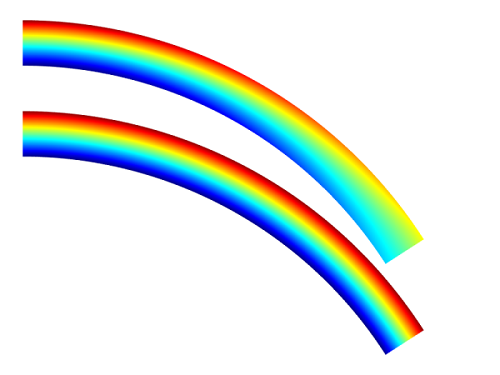
Cauchy and Second Piola-Kirchhoff stress for an initially straight beam with constant bending moment.
Another stress measure that you may encounter is the First Piola-Kirchhoff stress. It is a multiaxial generalization of the nominal (or engineering) stress. The stress is defined as the force in the current configuration acting on the original area. The First Piola-Kirchhoff is an unsymmetric tensor, and is for that reason less attractive to work with.
Sometimes you may also encounter the Kirchhoff stress. The Kirchhoff stress is just the Cauchy stress scaled by the volume change. It has little physical significance, but can be convenient in some mathematical and numerical operations.
Unfortunately, even without a rotation, the actual values of all these stress representations are not the same. All of them scale differently with respect to local volume changes and stretches. This is illustrated in the graph below. The xx-component of several stress measures are plotted at the fixed end of the beam, where the beam axis coincides with the x-axis. In the center of the beam, where strains, and thereby volume changes are small, all values approach each other. So for a case with large rotation but small strains, the stress representations can be seen as pure rotations of the same stress tensor.
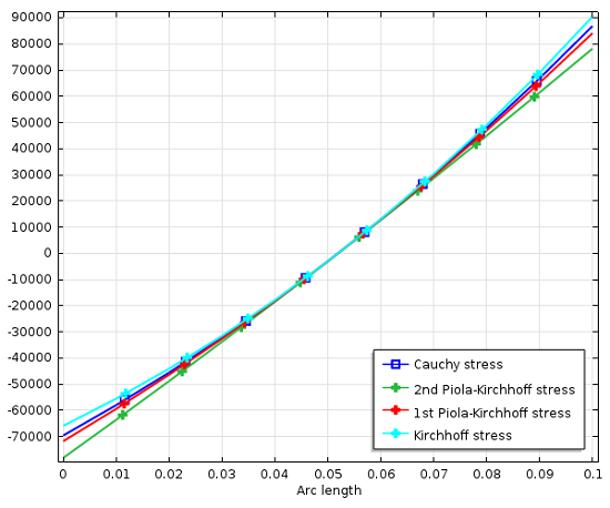
The distribution of axial stress at the fixed end of the beam.
If you want to compute the resulting force or a moment on a certain boundary, there are really only two possible choices: Either integrate the Cauchy stress over the deformed boundary, or integrate the First Piola-Kirchhoff stress over the same boundary in the undeformed configuration. In COMSOL Multiphysics this corresponds to selecting either “Spatial frame” or “Material frame” in the settings for the integration operator.
Strain Measures
When investigating the uniaxial tensile test above, three different representations of the strain were introduced. It is possible to generalize all of them to multiaxial cases, but for the true strain this is not trivial. It has to be done through a representation in the principal strain directions because that is the only way to take the logarithm of a tensor. The general tensor representation of the logarithmic strain is often called Hencky strain.
There are also many other possible representations of the deformation. Any reasonable representation however, must be able to represent a rigid rotation of an unstrained body without producing any strain. The engineering strain fails here, thus it cannot be used for general geometrically nonlinear cases. One common choice for representing large strains is the Green-Lagrange strain. It contains derivatives of the displacements with respect to the original configuration. The values therefore represent strains in material directions, similar to the behavior of the Second Piola-Kirchhoff stress. This allows a physical interpretation, but it must be realized that even for a uniaxial case, the Green-Lagrange strain is strongly nonlinear with respect to the displacement. If an object is stretched to twice its original length, the Green-Lagrange strain is 1.5 in the stretching direction. If the object is compressed to half its length, the strain would read -0.375.
An even more fundamental quantity is the deformation gradient, \mathbf F, which contains the derivatives of the deformed coordinates with respect to the original coordinates, \mathbf F = \frac{\partial \mathbf x}{\partial \mathbf X}. The deformation gradient contains all information about the local deformation in the solid, and can be used to form many other strain quantities. As an example, the Green-Lagrange strain is \frac{1}{2} (\mathbf{F}^T \mathbf F-\mathbf I). A similar strain tensor, but based on derivatives with respect to coordinates in the deformed configuration, is the Almansi strain tensor, \frac{1}{2} ( \mathbf I-( \mathbf{F} \mathbf F^T)^{-1}). The Almansi strain tensor will then refer to directions fixed in space.
Conjugate Quantities
A general way to express the continuum mechanics problem is by using a weak formulation. In mechanics this is known as the principle of virtual work, which states that the internal work done by an infinitesimal strain variation operating on the current stresses equals the external work done by a corresponding virtual displacement operating on the loads. The stress and strain measures must then be selected so that their product gives an accurate energy density. This energy density may be related either to the undeformed or deformed volume, depending on whether the internal virtual work is integrated over the original or the deformed geometry.
In the table below, some corresponding conjugate stress-strain pairs are summarized:
| Strain | Stress | Symmetry | Volume | Orientation |
|---|---|---|---|---|
| Engineering Strain (based on deformed geometry); True strain; Almansi strain | Cauchy (True stress) | Symmetric | Deformed | Spatial |
| Engineering Strain (based on deformed geometry); True strain; Almansi strain | Kirchhoff | Symmetric | Original | Spatial |
| Deformation gradient | First Piola-Kirchhoff (Nominal Stress) | Non-symmetric | Original | Mixed |
| Green-Lagrange strain | Second Piola-Kirchhoff (Material Stress) | Symmetric | Original | Material |
In the Solid Mechanics interface in COMSOL Multiphysics, the principle of virtual work is always expressed in the undeformed geometry (the “Material frame”). Green-Lagrange strains and Second Piola-Kirchhoff stresses are then used. Such a formulation is sometimes called a “Total Lagrangian” formulation. A formulation that is instead based on quantities in the current configuration is called an “Updated Lagrangian” formulation.
Additional Resources on Stresses and Strains
- More on the mathematical definition of various stress measures
- Further details on various strain measures here and here
- Conjugate stress-strains pairs and virtual work
- A publication on possible pitfalls when not respecting the conjugacy rules


Comments (7)
Ivar Kjelberg
November 22, 2013Thanks Henrik for these precisions
For those desiring to get more details about the different stresses, in a very close to COMSOL notation, I can only suggest to read the excellent and recent two books of “Tadmor, Miller and Elliot”: “Continuum Mechanics and Thermodynamics” & “Modelling Materials” (Cambridge University Press 2012)
I find your blogs so essential that I believe you should assemble them and distribute them, by physics, as e-booklets 😉
Ivar
Nagi Elabbasi
November 22, 2013Thanks Henrik!
Sandeep Ramini
December 15, 2017Thanks Henrik 🙂
COMSOL blogs comes to my rescue whenever I need to understand complex concepts in a simplest way possible. A big thanks to COMSOL team!!
Josh Thomas
March 1, 2018Henrik,
You have said it is important to make sure we know “In what form your analysis software expects it for a specific material model.”
So, would you mind commenting on which form COMSOL expects material properties? For example, can we assume that sigmags (Yield Strength) and sigmah (Hardening functions) material properties should be input in the form of true stress and true strain?
Thanks,
Josh Thomas
AltaSim Technologies
Henrik Sönnerlind
March 1, 2018Hi Josh,
That would depend on the material model, so you have to check with the documentation. But for your specific question, pertaining to large strain plasticity, the answer is: Yes, it is true (Cauchy) stress vs. true (logarithmic) strain.
For most other material models, you can expect 2nd Piola-Kirchhoff stress vs. Green-Lagrange strain.
Regards,
Henrik
K g v kalyan Kumar
July 24, 2020what is the expression that is used for true strain in comsol?
Timo Rikmanspoel
March 30, 2021Hi Henrik,
Currently I am working with 3D printing and my goal is to model the scaffolds I print in COMSOL. The scaffolds consist of fibers in different directions.
The main goal of my model is to examine the tensile strength properties of the scaffolds (Yield strenght, Young’s modulus) and obtain a stress/strain curve as close as possible to experimental data.
In COMSOL there are a lot of options for the stress and strain to apply (e.g. first principal strain or second piola-kirchhoff stress). Can you help me with which stress and strain I can choose the best for my model?
Thanks,
Timo Rikmanspoel