Problem Description
When I look at the Solver Log of a time dependent model, I see that the NLFail column has non-zero entries:
| Step | Time | Stepsize | Res | Jac | Sol | Order | Tfail | NLfail | LinErr | LinRes |
|---|---|---|---|---|---|---|---|---|---|---|
| 0 | 0 | -out | 2 | 3 | 2 | 0 | 8e-14 | 3.5e-15 | ||
| 1 | 0.1 | 0.1 | 11 | 5 | 11 | 1 | 0 | 1 | 2.6e-16 | 2.4e-16 |
| ... | ... | ... | ... | ... | ... | ... | ... | ... | ... | ... |
What does this mean?
When solving a time dependent model, I get an error message similar to:
Nonlinear solver did not converge.
Maximum number of Newton iterations reached.
Time : 0.15582918651998362
Last time step is not converged.
What changes can I make to the solver settings to fix this?
Solution
The time dependent solver is computing the solution to a possibly nonlinear system of equations at each timestep via a set of iterative techniques based upon Newton's method. If these iterative techniques fail at any timestep, the NLFail column will get incremented. These Newton's method techniques for solving a nonlinear system of equations evaluate a function, as well as its derivative, at every timestep. This derivative is also known as the Jacobian and is relatively expensive to compute. Therefore the software will try to minimize reevaluating the Jacobian, by default. If the nonlinear solver has difficulty converging, it will reduce the requested timestep size and try to compute the solution. When the timestep is reduced, the Tfail column is incremented. This is a good approach if the solution fields vary rapidly in time.
However this can be a suboptimal approach, or may not work at all, if the model has strong nonlinearities. Such nonlinearities can arise as a consequence of material properties being a function of the solution, or due to feedback equations such as, for example, when using the Current- or Power-type Terminal conditions in the Electric Currents physics interface.
- Note: Before making any of the solver changes described below, make certain that your model is well-posed. Examine the nonlinearities in your model and any feedback conditions and try to estimate what kind of response they will produce for your given inputs. If the solution shoots off to infinity due to positive feedback, for example, the solver will not be able to capture this. A non-converging model can often be a sign of an incorrectly, or incompletely, set up model. If you are modeling a problem with wave-like solutions, first make sure to apply the settings described in Knowledge Base 1118: Resolving time-dependent waves and also review Knowledge Base 1244: Solving Wave-Type Problems with Step Changes in the Loads. If you are not solving a wave-like problem, and if the non-convergence is happening when a load or boundary condition is changing abruptly in time, use Events as described in Knowledge Base 1245: Solving Models with Pulsed Loads in Time. Always make certain that your boundary conditions and loads are in agreement with your initial conditions, as discussed in Knowledgebase 1172: Solving time dependent models with inconsistent initial values.
The resolution can be to update the Jacobian on every iteration that the nonlinear solver takes as it tries to compute the solution at each timestep. To do so, expand out the Study settings and go to the Time-Dependent Solver branch, Fully Coupled subfeature, Method and Termination section. Modify the Jacobian update: to be On every iteration rather than Minimal, as shown below. This change can often be enough.
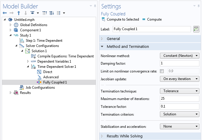
Modified settings in the Fully Coupled feature.
However, sometimes the nonlinear problem at every timestep is so strongly nonlinear that the Newton's method is still not able to converge, even with an updated Jacobian. The next setting to change is the Maximum number of iterations, which has a default value of 4 . Increase this to 25, or higher. Next, adjust the Tolerance factor: setting. Its default value of 1 means that the relative tolerance setting is being used, as specified in the Time Dependent Study Step. The default value of the relative tolerance is 0.01 and the Tolerance Factor: multiplies this number, so setting the Tolerance factor: to 0.1 in this case would result in a relative tolerance of 0.001 used for the nonlinear problem at each timestep. Thus, as you tighten the time-dependent solver relative tolerance setting, you can usually relax the tolerance factor.
If your model is still not converging, change the Nonlinear method: setting from Constant (Newton) to Automatic (Newton) which implements a damped Newton's method approach. This automatically updates the Jacobian and uses a dynamic damping term, it is therefore more computationally expensive. The Automatic highly nonlinear (Newton) is similar, but starts with more damping, and will be slower but more likely to converge.
Your model may, by default, be using a segregated approach. This is often the case when solving multiphysics problems and is usually reasonable since the strong nonlinearities often affect just one of the physics in the model. Within the segregated solver each segregated step represents the solution to a different physics and is being solved separately, again using some variation of Newton's method. You can make similar modifications as described above, but just to one segregated step, as motivated by the nonlinearities present. That is, if a material or feedback nonlinearity is present in only one physics, you probably only need to modify the settings for that physics, as shown in the screenshot below.
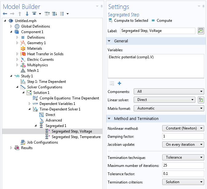
Modified settings in the Segregated Step feature.
If you are solving a multiphysics problem and suspect that there are strong nonlinearities between the physics, then switch from the segregated to fully coupled approach, as described in Knowledge Base 1258: Understanding the Fully Coupled vs. Segregated approach. You may still need to adjust the settings as described earlier.
If you are primarily observing that the Tfail column in the solver log is being incremented often, enable the Nonlinear controller within the Time Stepping settings as shown in the screenshot below. This will enable more efficient time-step control in the BDF method, especially for highly nonlinear models. Note that the Tfail column can get incremented even for a model without nonlinearities, in which case it is better to tighten the solver relative tolerance.
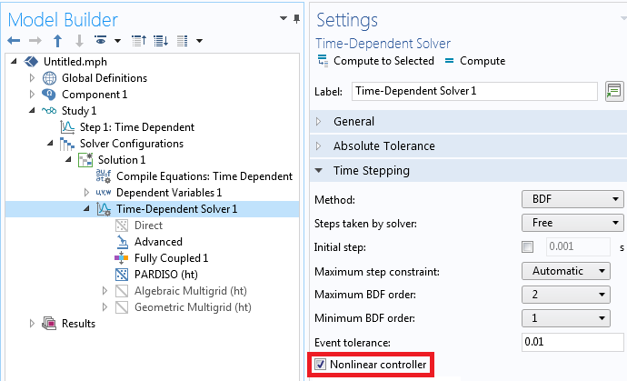
Enabling the nonlinear controller.
Lastly, keep in mind that you will always need to perform both a relative tolerance refinement study, as described here: Knowledge Base 1254: Controlling the Time-Dependent Solver Timesteps, and a mesh refinement study, as described here: Knowledge Base 1261: Performing a Mesh Refinement Study, to verify the accuracy of your model.
Recherche par catégorie
Messages d'erreur (64)Import (7)
Géométrie (11)
Physiques (11)
Solveur (38)
Installation (40)
Maillage (14)
Général (38)
Mécanique des structures (2)
Mécanique des fluides (2)
Post-traitement (4)
Export (1)
Dessin (1)
Informations produit (6)
Multiphysique (1)
Modèles utilisateurs (1)
Electromagnétisme (1)
COMSOL makes every reasonable effort to verify the information you view on this page. Resources and documents are provided for your information only, and COMSOL makes no explicit or implied claims to their validity. COMSOL does not assume any legal liability for the accuracy of the data disclosed. Any trademarks referenced in this document are the property of their respective owners. Consult your product manuals for complete trademark details.