Modeling with PDEs: Helmholtz Equation
Here in Part 7 of this course on modeling with partial differential equations (PDEs) in COMSOL Multiphysics®, you will learn how to use the PDE interfaces to model the Helmholtz equation for acoustics wave phenomena in the frequency domain. The predefined physics interfaces for modeling acoustic wave propagation make this easy and, for virtually all purposes, this is the recommended approach when working with acoustics. For educational purposes, this article will focus on how to derive the expressions for implementing low-reflecting boundary conditions by hand, and in the process of doing so, how to work with complex-valued quantities in the software. This will give you an appreciation for and a deeper understanding of how frequency-domain modeling is implemented in the Acoustics Module as well as in other add-on products used for wave propagation phenomena.
The Wave Equation
The wave equation is prevalent in many areas of engineering, including acoustics, structural dynamics, and electromagnetics. Let us see how we can use the mathematics interfaces in COMSOL Multiphysics® to model a scalar version of the wave equation that solves for one frequency at a time: the Helmholtz equation. Before studying the Helmholtz equation we will need some background on the wave equation used for pressure acoustics.
We can start by recalling the Coefficient Form PDE:

This equation template can be found among the Mathematics interfaces in the Model Wizard.
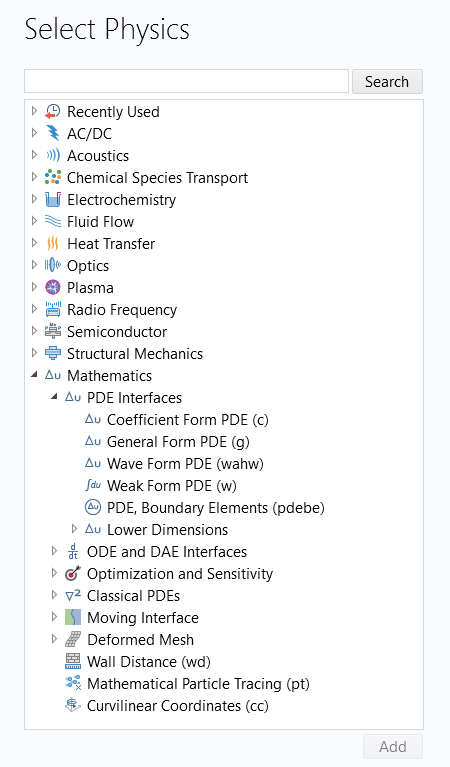
The Mathematics interfaces in the Model Wizard, under which you can find the Coefficient Form PDE interface.
For more information about using the Coefficient Form PDE interface, see the Coefficient Form PDE section of the previous Learning Center article on modeling diffusion-type equations.
If we keep the second-order time-derivative term, but ignore some of the other terms, we get the wave equation

This equation, in different forms, can be used to represent acoustic waves, electromagnetic waves, or elastic waves.
Let us now consider pressure acoustics. For acoustics waves, the dependent variable is a scalar quantity representing the acoustic pressure. The wave equation takes on a particularly simple form:

where  is the pressure field,
  is the fluid density, and
  is the speed of sound.
This equation is available as a built-in option under the Acoustics branch in the Model Wizard, under the Pressure Acoustics branch. If you have the Acoustics Module, then there are several different versions of this equation available. In this article we will only consider the transient and frequency domain version of the equation. The Frequency Domain version of the Pressure Acoustics interface (shown in the image below) is available in the core COMSOL Multiphysics® package as well as in the Acoustics Module. When using this interface, you will find some basic functionality in the core package and many more advanced options in the Acoustics Module. It is important to emphasize that it is much easier to solve for Pressure Acoustics using the built-in physics interface for pressure acoustics. However, for the purposes of this article, we are looking to understand the underlying techniques and PDEs by using the mathematics interfaces.
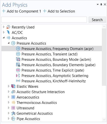
The Pressure Acoustics, Frequency Domain interface is selected in the Add Physics window.
We can compare the pressure acoustics formulation with the Coefficient Form PDE and note that:


An extended version of the pressure acoustic equation takes on this form:

where  is a monopole source density and
  is a dipole source density.
Again, we can compare this with the Coefficient Form PDE and see that:


This gives another case where the conservative source term is useful.
For an example of solving the transient wave equation, see the Transient Gaussian Explosion tutorial model. Note, however, that this example uses the built-in interfaces of the Acoustics Module and not any of the Mathematics interfaces.
Helmholtz Equation
We will keep working with the pressure acoustics equation but now move from the time domain to the frequency domain. To do so, first assume a sinusoidal (also known as harmonic) pressure field at a frequency,  , or angular frequency
  , and real-valued pressure amplitude
  :
:

When working with one frequency at a time (or in the frequency domain), it is convenient to instead work with a complex-valued pressure.
Using complex arithmetic, we instead assume a complex-valued pressure:

where we can get the original equation by taking the real part

Similarly, we need to require that the source term is harmonic and varying at the same frequency:

Insert these complex-valued expressions into the pressure wave equation and derive the Helmholtz equation as follows:


Matching coefficients with the Coefficient Form PDE gives us:


The term  in the Coefficient Form PDE is therefore sometimes called a Helmholtz term.
Now, let us change back to using  as the dependent variable and introduce the wave number
  according to
  . Then we can write

and Helmholtz equation takes the following form:

We also have boundary conditions associated with this equation: the Neumann boundary condition:

and the Dirichlet condition:

The figures below show the Parameter and Coefficient Form PDE settings for this version of the Helmholtz equation, respectively.
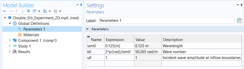
The associated parameters used for the Helmholtz equation.
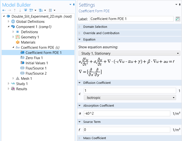
The Coefficient Form PDE node settings for the Helmholtz Equation.
Note that when moving from the time-dependent acoustic equation to the Helmholtz equation, its frequency-domain counterpart, we are solving a stationary PDE and will use a Stationary study.
Example: The Double-Slit Experiment
Let us now look at a classical application of the Helmholtz equation, the double-slit experiment. Here, we assume that the waves are acoustic pressure waves. However, we are not paying attention to the speed of sound or the density. Instead, to keep things simple, we will assume a wave vector as the only input to the equation. You can think of this as assigning the value 1.0 to both the speed of sound and the fluid density.
In our example, a plane wave is entering the computational domain from the left. Some portion of the waves will be reflected off the wall and some portion will be passing through the double slit. An interference pattern will be seen on the screen and there will be outgoing waves leaving the domain on the right. For simplicity, we will assume that the screen is transparent to the wave. The difficult part of setting up this type of analysis is defining the boundary conditions. The boundary condition on the left will need to accommodate both the incoming wave and the reflected wave. In addition, we will need to allow the waves to leave the domain on the right.
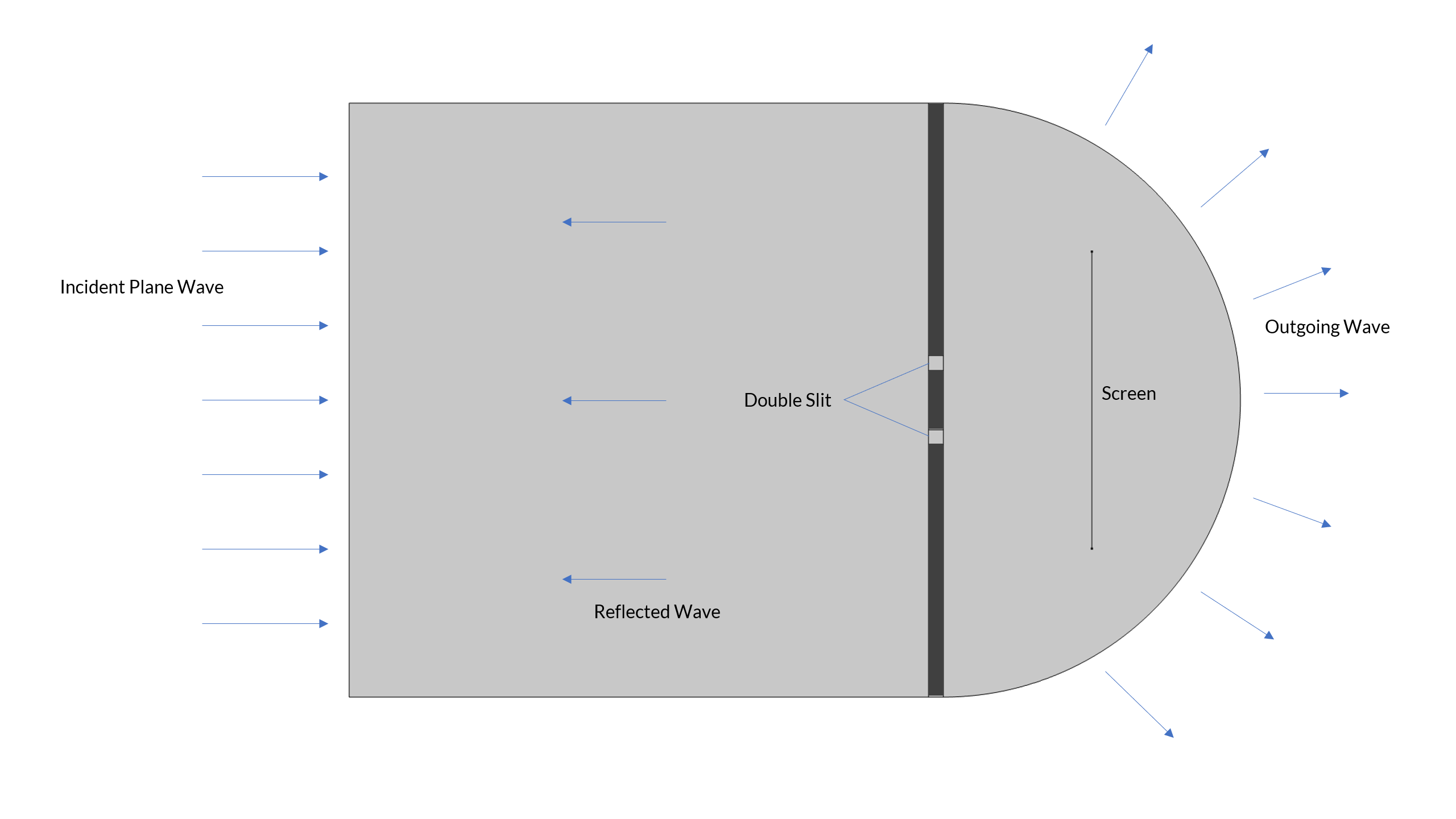 A geometric figure with the double slit labeled and blue arrows showing the incident plane wave, reflected wave, and outgoing wave.
The double-slit experiment setup.
Plane Wave Solution
To understand how to apply suitable boundary conditions it is useful to first review a very important closed-form solution to the source-free Helmholtz equation for plane waves. This solution is easy to write down and interpret.
The plane wave solution to Helmholtz equation in free space takes the following form:

where  is the wave vector
 is the wave number
 is a spatial coordinate vector
 is a constant wave amplitude
The alternative solution,  , with a wave vector of opposite sign, is also a plane wave solution to the Helmholtz equation. We can pick any one of these two solutions for the derivations below.
Note that in order to retrieve the time-dependent solution we can compute:

where the subscript  indicates a real-valued quantity.
Let us check that the plane wave solution really satisfies the Helmholtz equation.
If we insert the plane wave expression into:

where we will further assume that 
we get

Now, we need to use the following two identities for the gradient and divergence operators:


Going back to Helmholtz equation, we get that:
becomes

which shows that the equation is indeed satisfied by the plane wave solution.
Radiation Boundary Conditions
At the boundaries we will need a so-called radiation boundary condition, also known as a low-reflecting boundary condition. In their simplest form they can be derived from the plane wave solution as follows.
Assume that at a boundary the solution is the sum of a known incident wave,  , and and an unknown scattered wave,
  :
:

Furthermore, we will assume that the incident and scattered waves are propagating in opposite directions. This allows us to set:


so that, with an arbitrary choice of sign:


where is the wave number and  is the outward normal vector to the boundary surface.
Note that this is an approximation and we will get unwanted reflections if there are components of the wave with a wave vector that is not normal to the surface. Such unwanted reflections are handled in the Acoustics Module by more sophisticated built-in radiation conditions and perfectly matched layers (PMLs). For our purposes, the simplified approach presented here will suffice.
We now need to fit this superposition of an incident and a scattered wave to the Neumann boundary condition, assuming :

We see that in order to do so we need to calculate  on the boundary.
We have that:


We can write this in terms of the original incident and scattered fields:


and we get:

Since we do not know the scattered wave, we need to formulate this gradient in terms of the known quantities, which are the dependent variable and the incident wave  . This way, we can use the expressions in the Neumann boundary condition.
We can do so as follows:

Now, multiplying with the normal vector , we get:

To make it easier to identify coefficients with the Neumann boundary condition for the Coefficient Form PDE, we can write this as:

If we compare this expression with
we see that


Note that for a boundary with no incident wave we have:

In our double-slit experiment model we use an incident wave that is traveling from the left to right (as shown in the picture of the setup above), which corresponds to the positive x direction. Furthermore, we assume the wave has amplitude  , in which case we have:


The negative sign is to keep the sign convention consistent with the earlier definition of a plane wave. However, the sign does not matter that much in this case since picking the other sign will just reverse the meaning of time and the direction of the wave vector. Since either direction is a valid solution in the frequency domain, both will give the same result. However, if you run an animation you will see that changing the sign will flip the direction of propagation or, equivalently, change the direction of time.
The figures below show the settings for the ingoing and outgoing boundary conditions.
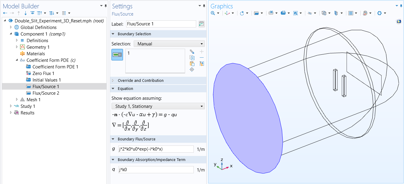 The COMSOL Multiphysics UI showing the Model Builder with the Flux/Source 1 boundary condition selected, the corresponding Settings window, and the double-slit model in the Graphics window.
The Flux/Source boundary condition settings for the boundary with an incident wave traveling from negative to positive x values.
The COMSOL Multiphysics UI showing the Model Builder with the Flux/Source 1 boundary condition selected, the corresponding Settings window, and the double-slit model in the Graphics window.
The Flux/Source boundary condition settings for the boundary with an incident wave traveling from negative to positive x values.
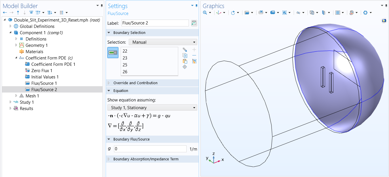 The COMSOL Multiphysics UI showing the Model Builder with the Flux/Source 2 boundary condition selected, the corresponding Settings window, and the double-slit model in the Graphics window with more 3D visuals.
The Flux/Source boundary condition settings for the boundary with an outgoing wave.
The COMSOL Multiphysics UI showing the Model Builder with the Flux/Source 2 boundary condition selected, the corresponding Settings window, and the double-slit model in the Graphics window with more 3D visuals.
The Flux/Source boundary condition settings for the boundary with an outgoing wave.
Meshing and Solving
When solving the Helmholtz equation, it is important that you make the mesh fine enough to resolve the wave oscillations. As a rule of thumb, the mesh should have 5 to 6 second-order elements per wavelength. However, in this example we will use 4 second-order elements per wavelength to make the model computationally less demanding. At this mesh density, the interference pattern starts to show and corresponds fairly closely to the results of using a finer mesh. The solver used is a geometric multigrid method with a so-called shifted Laplacian preconditioner, where a good value of the shift was found for the shift coefficient 0.8. For more information on this solver, see the COMSOL Multiphysics Reference Manual. Note that for the Pressure Acoustics, Frequency Domain interface in the Acoustics Module, the suitable solver settings are available as predefined solver suggestions; because of this, there is usually no need to change the solver settings.
In this example, the computation time is about 1 hour on a moderately powerful workstation and requires about 31 GB of RAM. If you do not have access to a powerful enough computer, you can download and use the corresponding 2D model provided in this article. The 2D model takes 2 seconds to solve and requires about 1.5 GB of RAM.
 The COMSOL Multiphysics UI with Mesh 1 selected in the Model Builder window with the settings open and the meshed double-slit model in the Graphics window.
The mesh needs to be fine enough to resolve the wave oscillations, in this case about l/4 where l is the wavelength.
The COMSOL Multiphysics UI with Mesh 1 selected in the Model Builder window with the settings open and the meshed double-slit model in the Graphics window.
The mesh needs to be fine enough to resolve the wave oscillations, in this case about l/4 where l is the wavelength.
Results
The results show the classical interference pattern behind the slits. The amplitude drops significantly behind the slits and the amplitude in front of the slits are further increased by the fact that most of the wave is reflected from the wall with the slits.
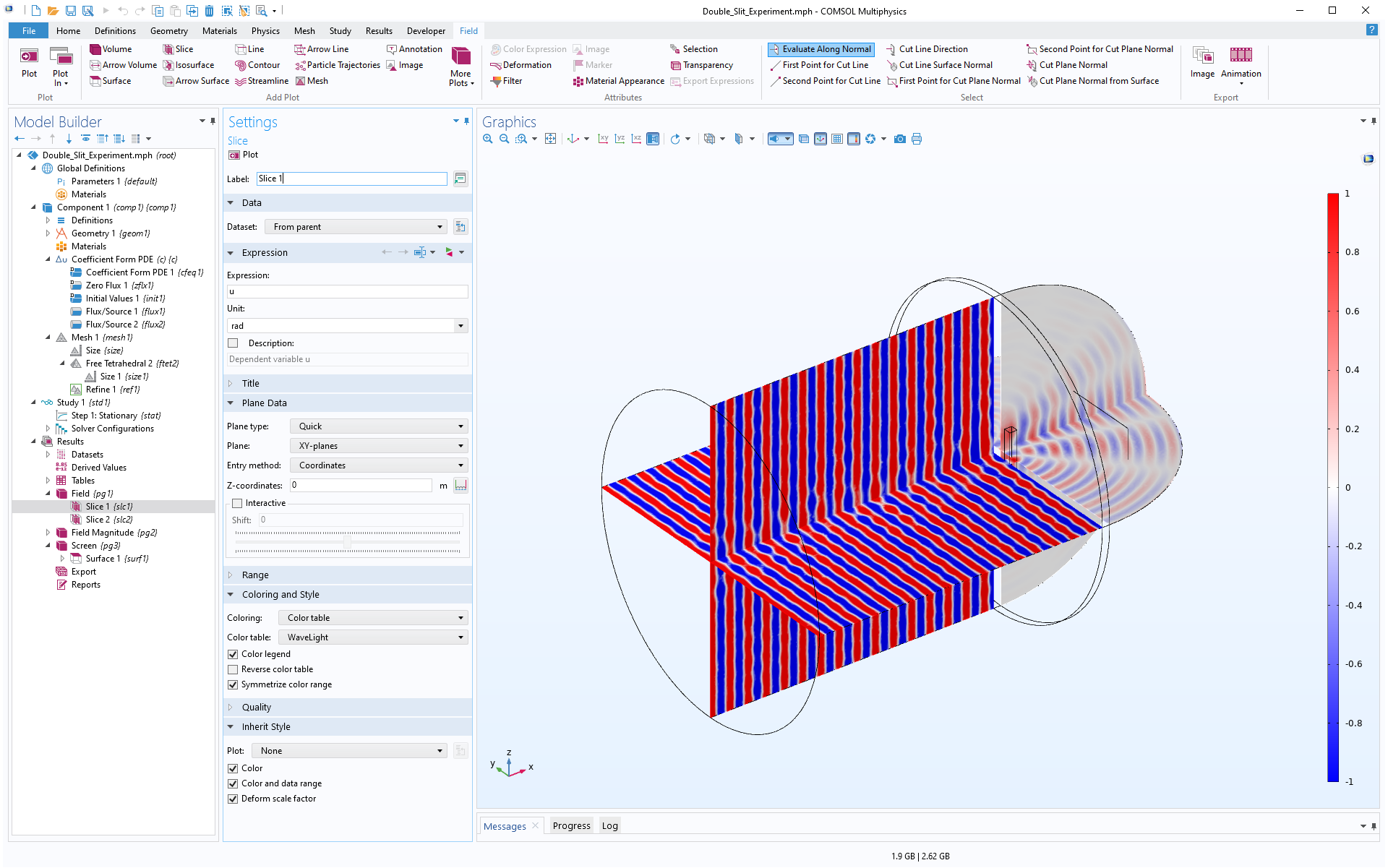 The COMSOL Multiphysics UI showing the Model Builder with Slice 1 selected, the corresponding Settings window, and the model in the Graphics window.
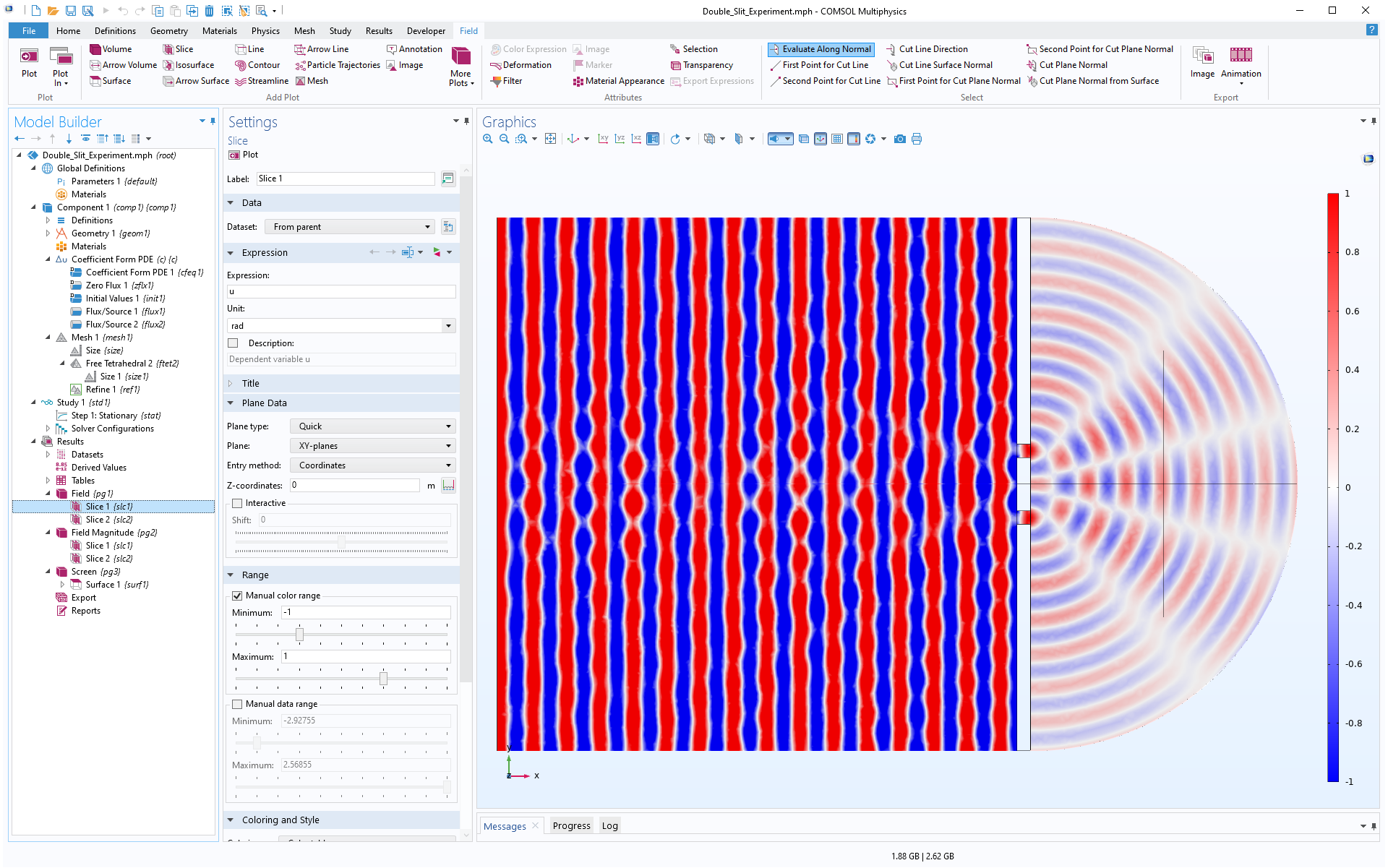 The COMSOL Multiphysics UI showing the Model Builder and Settings windows and a close-up of the model's interference pattern with blue and red amplitude maxima.
The interference pattern is more clearly visualized on the screen behind the slits. Here, we can see a few amplitude maxima in blue and red as well as a few amplitude minima in white. The blue versus red maxima reflect a sign change in the amplitude due to a 180 degree phase shift.
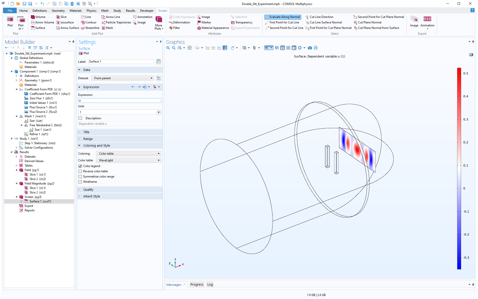 The COMSOL Multiphysics UI showing the Model Builder with Surface 1 selected, the corresponding settings, and the Graphics window showing an outline of the model and the interference pattern in blue, red, and white.
The interference pattern visualized on the screen.
The COMSOL Multiphysics UI showing the Model Builder with Surface 1 selected, the corresponding settings, and the Graphics window showing an outline of the model and the interference pattern in blue, red, and white.
The interference pattern visualized on the screen.
A corresponding 2D model shows more or less the same interference pattern, but with different amplitude. The 2D model, roughly speaking, corresponds to viewing the 3D model "from above", but with the slits extended indefinitely in the out-of-plane direction.
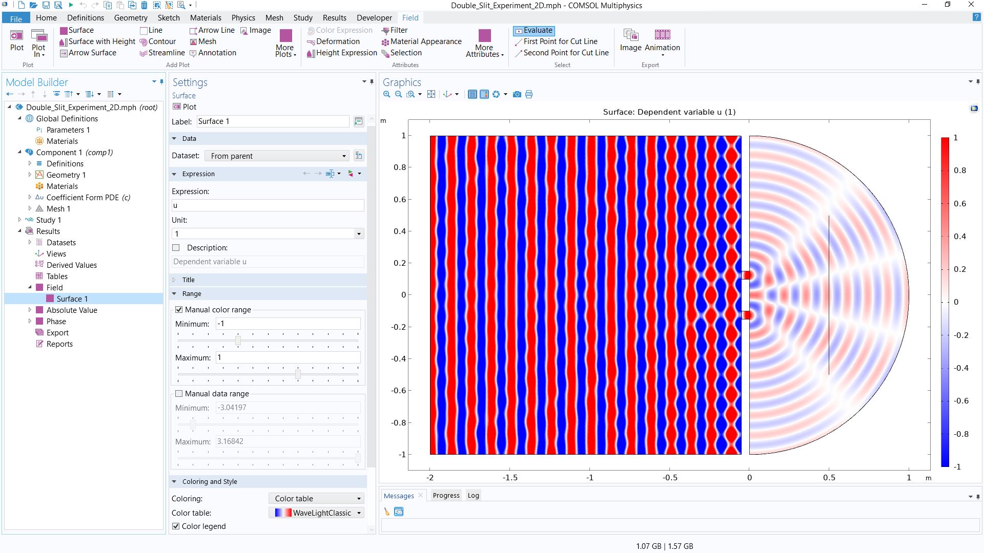 The COMSOL Multiphysics UI showing the Model Builder window with Surface 1 selected, the corresponding settings, and a close-up of the model's interference pattern for a 2D geometry, visualized as a square with red and blue lines increasing in waviness from left to right.
The same equation, but solved for a 2D geometry model.
The COMSOL Multiphysics UI showing the Model Builder window with Surface 1 selected, the corresponding settings, and a close-up of the model's interference pattern for a 2D geometry, visualized as a square with red and blue lines increasing in waviness from left to right.
The same equation, but solved for a 2D geometry model.
You can more easily, although less instructive, set up the same problem using the Pressure Acoustics, Frequency Domain interface and use the value 1.0 for both the fluid density and speed of sound. The corresponding model gives a near-identical result; however, because the Pressure Acoustics, Frequency Domain interface features a more sophisticated Cylindrical Wave Radiation boundary condition, there will be a slight difference in the results.
Complex-Valued Quantities
When modeling in the frequency domain, all the field quantities are complex valued. The argument, or angle, of the complex-valued field contains information about the phase of the wave, whereas the absolute value, or modulus, represents the wave amplitude.
You can use the following functions for the respective quantities in the expression field for any results plot:
abs()for the absolute valuearg()for the complex phase angle, or argumentreal()for the real partimag()for the imaginary part
The figures below show the absolute value and phase in the right part of the model.
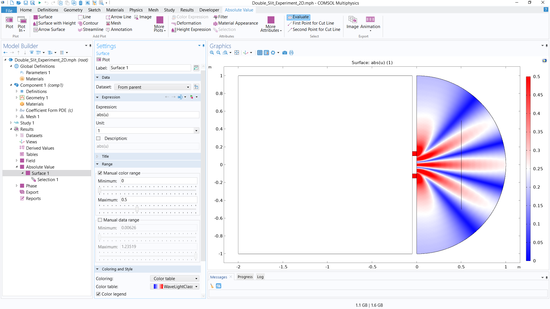 The COMSOL Multiphysics UI with Surface 1 selected and the Graphics window showing the absolute value of the field behind the double slit in blue, red, and white.
A visualization of the absolute value of the field behind the double slit.
The COMSOL Multiphysics UI with Surface 1 selected and the Graphics window showing the absolute value of the field behind the double slit in blue, red, and white.
A visualization of the absolute value of the field behind the double slit.
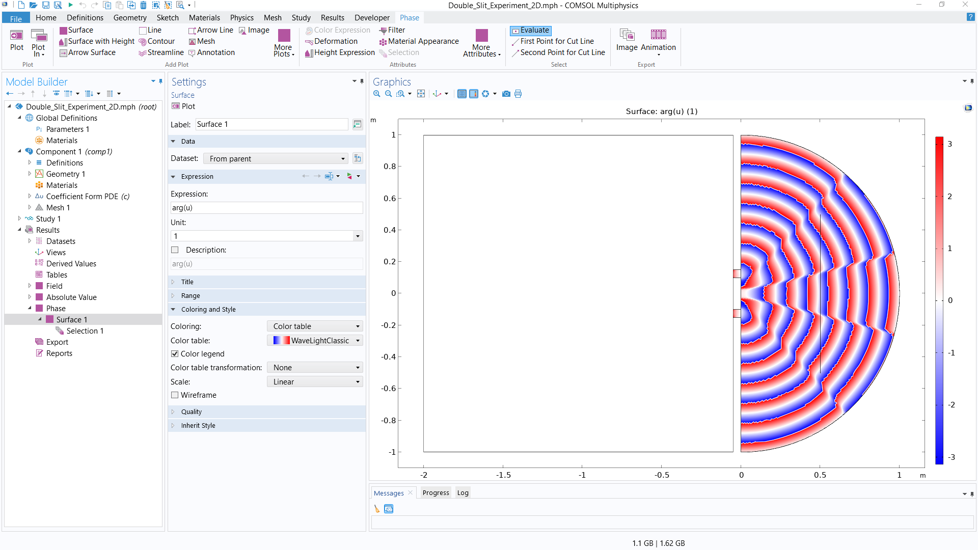 The phase angle visualization of the field behind the double slit, shown as a half-circle with blue, red, and white lines.
A visualization of the phase angle of the field behind the double slit.
The phase angle visualization of the field behind the double slit, shown as a half-circle with blue, red, and white lines.
A visualization of the phase angle of the field behind the double slit.
Eigenvalue Equations
COMSOL Multiphysics® provides a number of built-in interfaces, and associated study types, for eigenfrequency analysis. Without any add-on products, you have access to eigenfrequency analysis for acoustics as well as structural analysis. With certain add-on products, you have access to built-in interfaces for various types of eigenfrequency analyses, which can be used when working with, for example, electromagnetic and piezoelectric resonant devices. Depending on the application, the study types for these built-in interfaces have different names, such as Eigenfrequency, Eigenvalue, or Mode Analysis, but under the hood, they are all various formulations of eigenvalue equations.
For educational and research purposes, you can also use the Mathematics interfaces to solve your own eigenvalue equations, including the Helmholtz equation. To do so, you select the Eigenvalue study type instead of Stationary. For the Eigenvalue study types you should also set the number of eigenvalues and eigenfunctions that you would like the solver to find.
The eigenvalue version of the Coefficient Form PDE is:

where  is the eigenvalue and is the corresponding eigenfunction, also called eigenmode or just mode. By selecting the Eigenvalue study type you automatically get the Coefficient Form PDE of this form.
To understand where this equation is coming from, we perform a similar type of harmonic solution assumption, as in the derivation of Helmholtz equation. However, the convention used in this case is that the assumption has a real-valued exponent:

If we substitute this into the regular Coefficient Form PDE equation we get:

Now, we use that fact that:

and

By substituting these expressions we get the eigenvalue version of the Coefficient Form PDE (the factor  is cancelled out). Note that this is a quadratic eigenvalue equation and to get a conventional linear eigenvalue equation you simply set
  .
.
Since the software supports complex-valued arithmetic we will automatically get solutions that can be varying exponentially, sinusoidally, or both, corresponding to real, imaginary, and complex-valued eigenvalues, respectively. You can of course also solve systems of equations as a coupled system of eigenvalue equations.
For examples of modeling with eigenvalue equations, see our blog post on hearing the shape of a drum, the Isospectral Drums tutorial model, and the Conical Quantum Dot tutorial model.
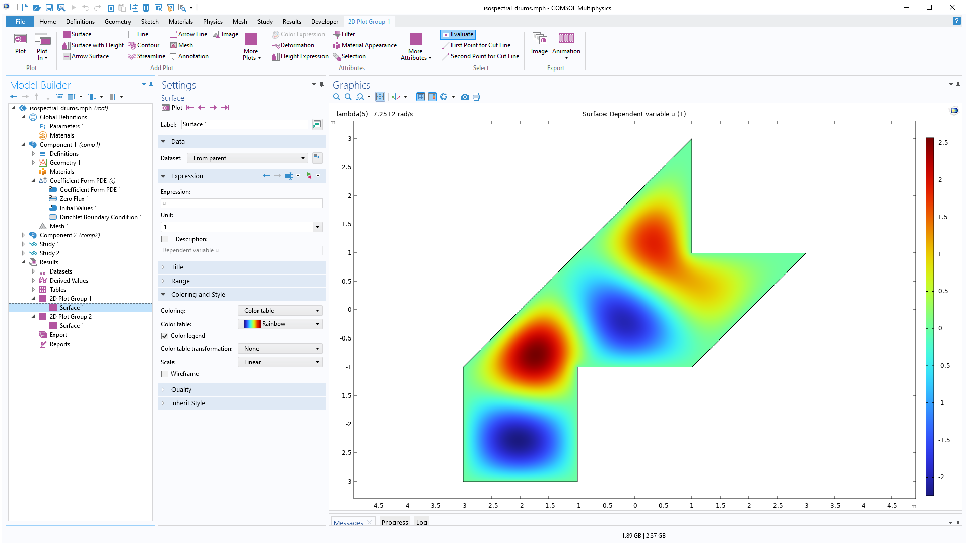 The COMSOL Multiphysics UI showing the Model Builder window with Surface 1 selected, the corresponding settings, and the Graphics window with a drum membrane model shown in bright green with two blue spots and two red spots.
One of the eigenmodes of a drum membrane with a polygonal boundary, from the Isospectral Drums tutorial model.
The COMSOL Multiphysics UI showing the Model Builder window with Surface 1 selected, the corresponding settings, and the Graphics window with a drum membrane model shown in bright green with two blue spots and two red spots.
One of the eigenmodes of a drum membrane with a polygonal boundary, from the Isospectral Drums tutorial model.
Further Learning
The files associated with this article include a 3D model without solution and a 2D model that compares results using the Coefficient Form PDE according to the "manual" derivations above and the built-in Pressure Acoustics, Frequency Domain interface. As an exercise, you can use the Coefficient Form PDE and implement the same radiation condition that you can find in the Pressure Acoustics, Frequency Domain interface, visible in the Equation section of the Cylindrical Wave Radiation boundary condition.
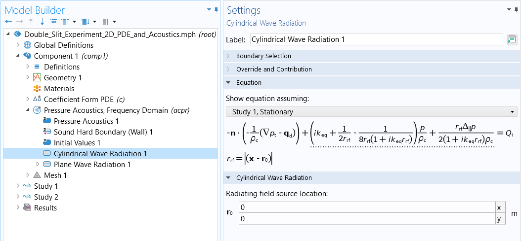 The Model Builder with the Cylindrical Wave Radiation 1 boundary condition selected and the corresponding Settings window with the Study 1, Stationary setting selected.
The Cylindrical Wave Radiation boundary condition.
The Model Builder with the Cylindrical Wave Radiation 1 boundary condition selected and the corresponding Settings window with the Study 1, Stationary setting selected.
The Cylindrical Wave Radiation boundary condition.
Envoyer des commentaires sur cette page ou contacter le support ici.