Modeling with PDEs: Poisson's and Laplace Equations
Here in Part 1 of this course on modeling with partial differential equations (PDEs), we begin with a quick introduction to using the general-purpose PDE interfaces in the COMSOL Multiphysics® software. You will learn how to use the interfaces, which are based on the finite element method (FEM) and boundary element method (BEM), for modeling with Poisson's and Laplace equations, respectively. Built-in mathematics interfaces are available for modeling these specific PDEs (i.e., the Laplace Equation interface and Poisson's Equation interface), however, in order to demonstrate how to implement your own custom equations we will not use them. You will also see an example of how to solve for the Newtonian gravity of the Earth–Moon system, since this does not have any corresponding built-in options in the software. However, the techniques used here are applicable in a much wider context. In subsequent parts, we will learn more about the mathematics interfaces and how to model more general PDEs as well as systems of PDEs.
The Mathematics Interfaces in COMSOL Multiphysics®
The mathematics interfaces can be found in the Model Wizard under Mathematics, as seen in the figure below.
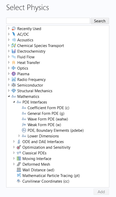
The Mathematics interfaces in the Model Wizard.
With these interfaces, you can solve various types of PDEs using different formulations and numerical methods. You can also use these interfaces to solve ordinary differential equations (ODEs) and other special types of equations. You can combine equations of different types to form a wide range of nonlinear equation systems, modeling all kinds of mathematical and physical processes. All of these interfaces, with the exception of some of those under the Optimization and Sensitivity and Moving Interface branches, are available as part of the core functionality in the software.
The Finite Element and Boundary Element Methods
In COMSOL Multiphysics®, the main method for solving PDEs is the finite element method and most of the mathematics and physics interfaces in the software are based on this method. However, in some cases it is beneficial to instead use BEM, frequently in combination with FEM. BEM uses a mesh on surfaces only, i.e., not in the computational volume. This is advantageous when the computational volume is large, which typically happens when the objects of interest are far apart. As a fun example of this, let us see how we can solve Laplace and Poisson's equation for the gravitational field of the Earth–Moon system (there is no corresponding built-in interface for this purpose). The Earth and the Moon are relatively far apart compared to their radii, which makes modeling the space that surrounds them suitable for BEM. To make things simple, we will assume classical stationary Newtonian gravity.
For electrostatics, corrosion, magnetostatics, and acoustics, there are dedicated physics interfaces that combine finite element and boundary element formulations. Since this is not the case for gravity, we will instead create custom equations and equation couplings by combining the finite-element-based Coefficient Form PDE interface with the boundary-element-based PDE, Boundary Elements interface. An additional benefit with the PDE, Boundary Elements interface is that it automatically covers an infinite computational volume. Note that in our case we will ignore any other celestial objects, but that the model presented here can easily be extended by adding the Sun or other objects.
Newtonian Gravity
Let us first introduce some notation. We will model gravity using partial differential equations. For this purpose, we need the gravitational vector field,  , having units of acceleration in SI units,
  . This field has three components in the x, y, and z direction:

To make computations easier and be able to formulate a scalar-valued PDE, we will also need the gravitational potential, which is a scalar field,  , with the somewhat unfamiliar unit of
  . We will see later how you can use the Mathematics interfaces to specify custom units and integrate them with the automatic unit handling capabilities in the software.
We will use the following notation from vector calculus:
 for the gradient of the scalar field.
 for the divergence of the vector field.
Gauss's law for gravitation is:  ,
,
where  is the gravitational constant and
  is the mass density. We can include the varying density due to the layering of, for example, the Earth's interior if we want to. However, in our example we will model the Earth and Moon with their average mass density values: 5515
  and 3340 , respectively. In the software, we will define these density values as Variables. This means you can change them to be functions of the coordinate variables x, y, and z, or, if you prefer spherical coordinates, r, theta, and phi.
The relationship between the gravitational field and the gravitational potential is:

By combining this we get the classical scalar equation for gravity, which is the following version of Poisson's equation:

The gravitational constant has the unit  and the density has the unit . Since these are multiplied together, the right-hand side of this equation has the unit
  or, equivalently,
  . Here, we will use the unit
  , which can be shown to also be equivalent to
  .
.
Since there is no mass density in free space,  and we can use the Laplace equation:

Note that the gravity vector field, , and the gravity potential, , have the same type of relationship as the electric field,  , and electric potential, , for electrostatics:

Also, there are dedicated physics interfaces for this that are available from the Model Wizard or the Add Physics window in the AC/DC branch, under the Electric Fields and Currents branch. In principle, we could use the Electrostatics interfaces for modeling gravity, but this would come with some drawbacks, such as unsuitable names for boundary conditions and the wrong units.
The Coefficient Form PDE Interface
One of the most important tools in COMSOL Multiphysics® for equation-based modeling is the Coefficient Form PDE interface. This equation template provides a powerful general interface for specifying linear and nonlinear equations, including the classical Poisson's and Laplace equations. Note that there are Mathematics interfaces specifically for Poisson's and Laplace equations. These interfaces are available from the Model Wizard under Mathematics > Classical PDEs and could have been used here. However, the goal of this article is to learn how to use the general-purpose PDE interfaces, such as the Coefficient Form PDE interface.
Using the notation of the user interface in the case where we have a scalar field  , the equation for the Coefficient Form PDE interface reads:

There are two important boundary conditions when using this interface. First, is the generalized Neumann boundary condition:
 ,
,
with  being the outward surface normal, which is used to model a boundary flux. The second is the Dirichlet boundary condition:

which is used to assign fixed values of the dependent variable on the boundary.
If we assume that we have just one dependent variable and that all materials are isotropic, then most of the coefficients are scalar quantities, but some are vector-valued as follows:
Scalars: 
Vectors: 
We will learn more about these coefficients in later articles. Note that for more general cases, the field quantities and coefficients can be vectors or matrices (tensors).
In the example of Newtonian gravity, we will now see how we can use the Coefficient Form PDE interface to define a PDE by simply matching the coefficients.
Poisson's Equation
In this example, we will only need the stationary version of the Coefficient Form PDE. In other words, we assume:

for all times of interest. This also means that we ignore the influence of the coefficients  and
and  .
.
We will not need many of the other coefficients. In our case, we have:


and end up with the equation (moving the negative sign in front):

To model our particular gravitational version of Poisson's equation, we will only use the coefficients  and
and  and leave all other coefficients with their default values (zero). Specifically for modeling the equation
we will have:
the dependent variable: 
the diffusion coefficient: 
the source term: 
We will shortly learn how to set this up from the beginning using the Model Wizard. To give you an idea on how this PDE will appear in the user interface, the corresponding Coefficient Form PDE interface is shown in the figure below.
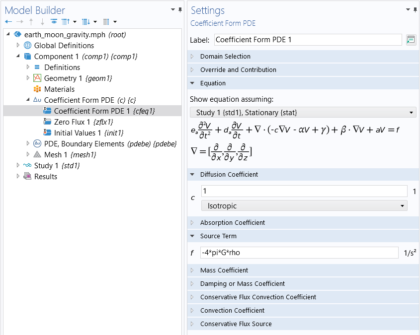
The gravity equation modeled using the Coefficient Form PDE interface.
where G and rho are defined as a parameter and a variable for the gravitational constant and density elsewhere in the model, respectively. The value of rho will be that of the Earth, 5515 ; and the Moon, 3340 , within the two spheres that we will use to represent these bodies.
The Model Wizard
Start by setting up a new model by, for example, selecting File > New. In the Model Wizard, select 3D as the space dimension, as shown in the figure below.
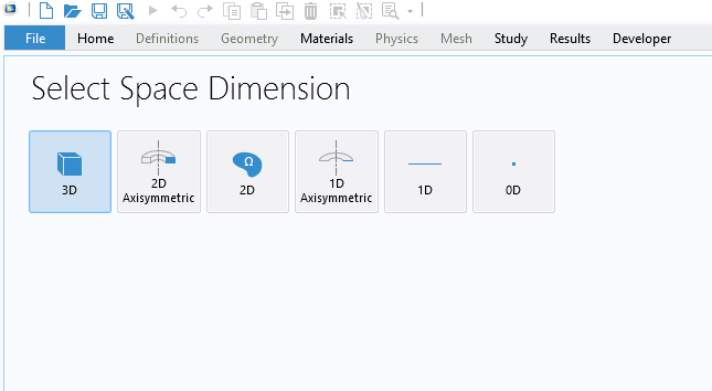
Selecting 3D for the space dimension in the Model Wizard.
For the next step, in the Model Wizard, select Mathematics > PDE Interfaces > Coefficient Form PDE. Change both the Field name and Dependent variables name to V, as shown below. For more general models, the Field name can be used to refer to an array or vector of dependent variables.
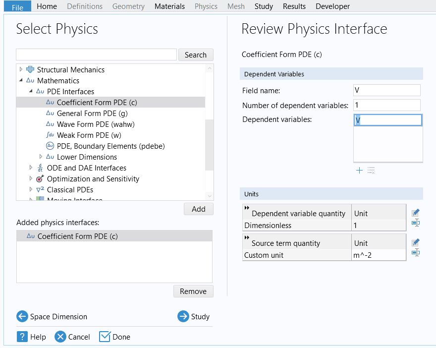 The Select Physics page with the Added physics interfaces field on the left and the Review Physics Interface window on the right showing the dependent variables and units.
The Select Physics page in the Model Wizard.
As shown in the image above, we need to change to custom units for the dependent variable quantity, which is the gravity potential with unit , as well as the source term with unit .
Click the Define Dependent Variable Unit button, available to the right of the Dependent variable quantity table in the Units section. Type J/kg, for the Unit, as shown here:
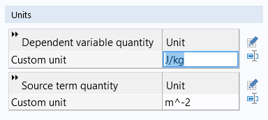
The Custom unit settings for the Dependent variable quantity.
Click the Define Source Term Unit button, available to the right of the Source term quantity table in the Units section. Type J/(m^2*kg), for the Unit, as shown in the figure below.
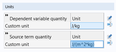
The Custom unit settings for the Source term quantity.
For the next step, in the Model Wizard, select Stationary for the study type.
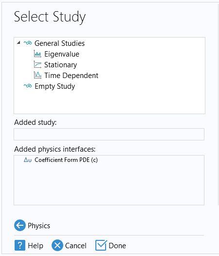
The Select Study page of the Model Wizard.
Click Done to enter the Model Builder 3D workspace.
Using the Coefficient Form PDE for Poisson's Equation
We need to define a few parameters for the radii of the Earth, r_earth, and the Moon, r_moon, as well as the distance to the moon, d_moon. There is a built-in parameter for the gravitational constant, G_const. For convenience, we redefined this as a parameter G. This is all shown in the figure below.
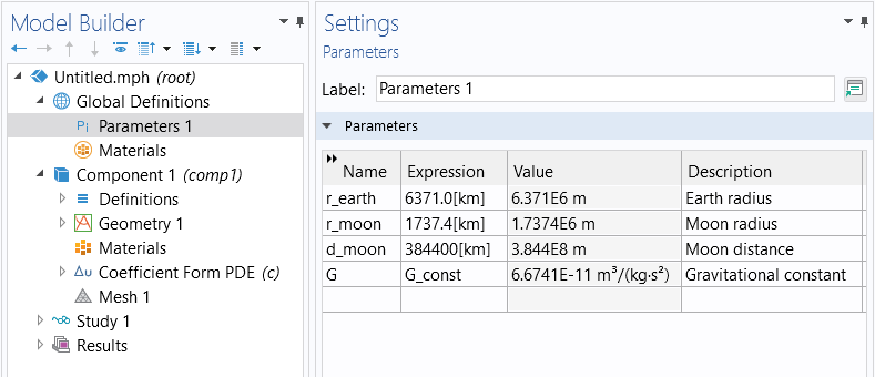
The parameters used in the example model.
The geometry simply consists of two spheres at the distance d_moon apart, as shown in the figure below.
 The COMSOL Multiphysics UI showing the Model Builder and Sphere settings window, with the geometry for the Earth–Moon system in the Graphics window.
The geometry model for the Earth–Moon system.
In the model, we have changed the length unit from m to km. Note that we do not need to enclose the two spheres in a volume mesh due to the fact that we will use a boundary element method for the gravity in space. This model could alternatively be defined as a 2D axisymmetric model.
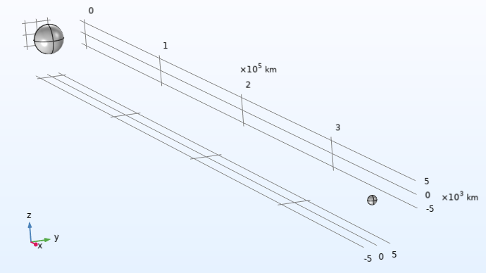
The Earth–Moon system modeled as two spheres with a length unit set to km.
The average density of the Earth and the Moon are defined as two domain variables with the same name, rho, taking different values in domain 1 (Earth) and domain 2 (Moon), as shown in the figures below.
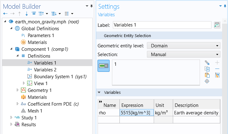
The variable for the average density of the Earth.
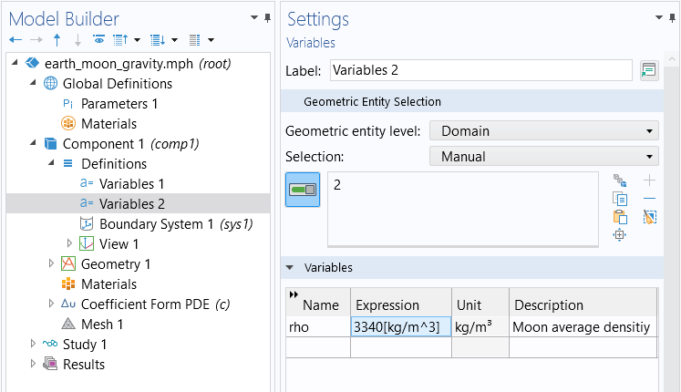
The variable for the average density of the Moon.
Note that you can make the expression for the varying density in space, as described earlier.
In the next step, define the coefficients for the Coefficient Form PDE settings as described earlier (also shown in the figure below).
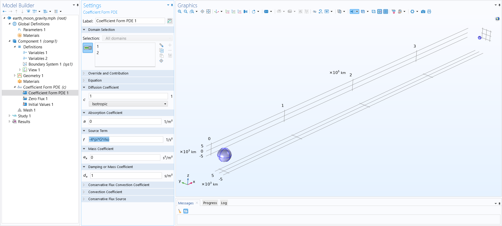 The COMSOL Multiphysics UI showing the Model Builder and the Coefficient Form PDE settings window, with the Earth–Moon system model in the Graphics window.
The Coefficient Form PDE settings for the Earth–Moon system.
This concludes the setup of the finite-element-based Coefficient Form PDE. In the next step we add a PDE, Boundary Elements interface.
Using the PDE, Boundary Elements Interface for Laplace Equation
Since we will model the Earth–Moon system as an idealized and isolated system, we do not want to impose unnecessary and artificial boundary conditions. We would like to view the system as situated in infinite free space without external disturbances. For this purpose, we will use the PDE, Boundary Elements interface. This interface will more or less automatically handle the infinite computational domain outside (and between) the Earth–Moon system.
The PDE, Boundary Elements interface covers a stationary PDE of the following form:

Notice that this form does not feature a source term, so we cannot use it to solve Poisson's equation. However, we can use it in free space since that is where the gravitational potential is governed by the Laplace equation:

In identifying the coefficients we see that:
the dependent variable:
the diffusion coefficient:
the absorption coefficient, or Helmholtz coefficient:
The PDE, Boundary Elements interface is available in the list of Mathematics interfaces. To add this interface, you can right-click Component 1 and select from the Add Physics window. The interface is available at: Mathematics > PDE Interfaces > PDE, Boundary Elements, as shown below.
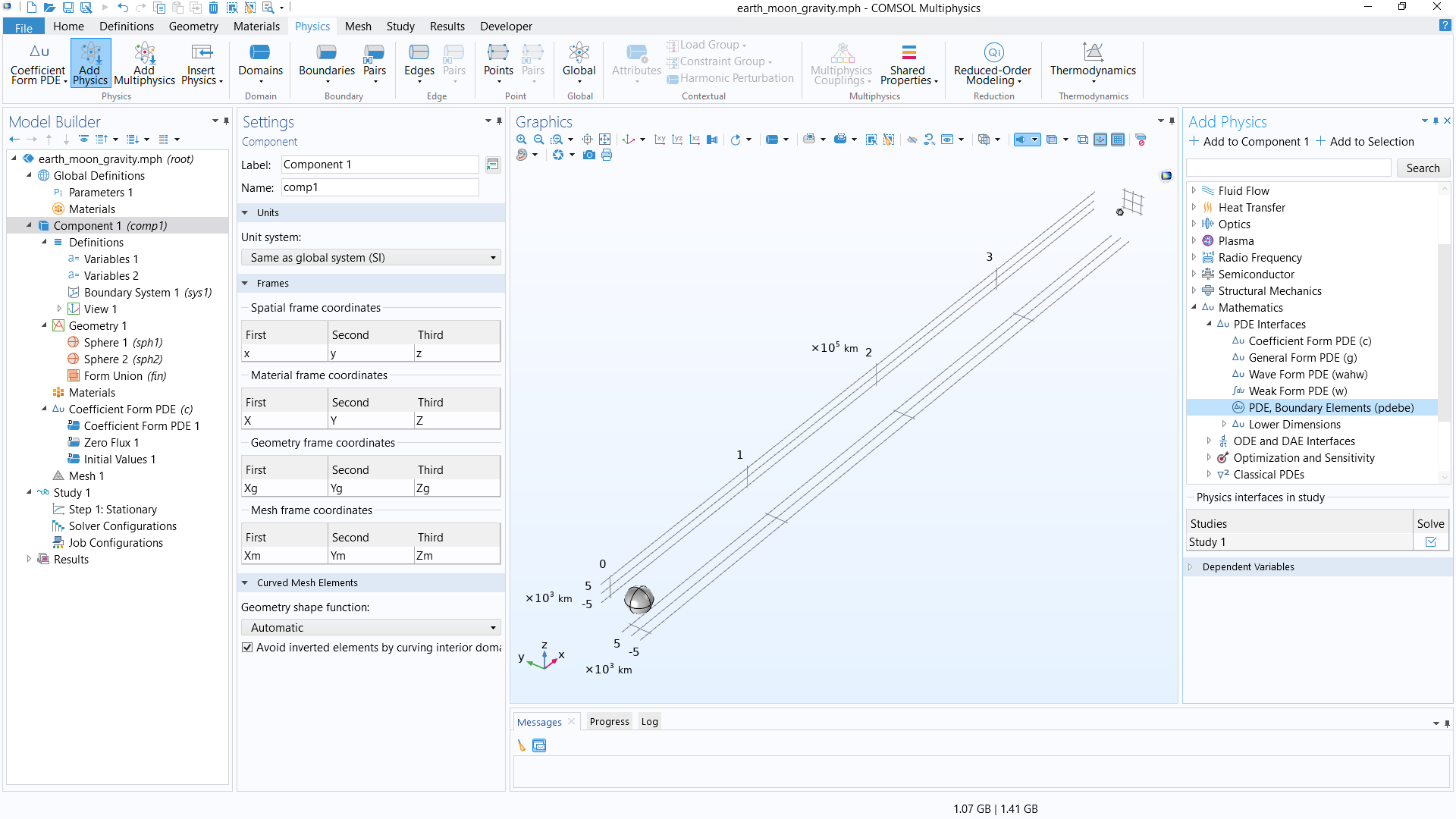 The COMSOL Multiphysics UI showing the Model Builder, Component settings, the Earth–Moon system in the Graphics window, and the Add Physics window with PDE, Boundary Elements highlighted.
The PDE, Boundary Elements interface is added to the model through the Add Physics window.
By default, domain 1 and 2 and the Infinite void domain are selected for the PDE, Boundary Elements. The Infinite void is COMSOL terminology for the space surrounding the spheres and all the way out to infinity. We need to remove domain 1 and 2 since we only want to apply the PDE, Boundary Elements in the Infinite void domain, as shown below.
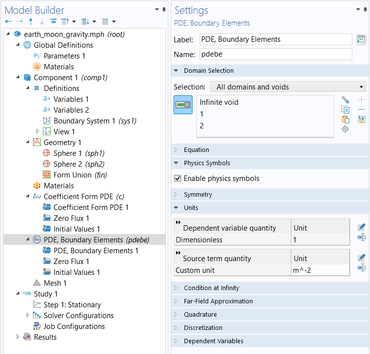
The domain selection for the PDE, Boundary Elements interface before deleting domains 1 and 2 from the geometry selection.
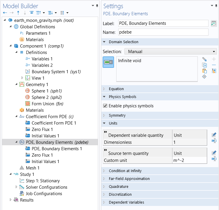
The domain selection for the PDE, Boundary Elements interface after deleting domains 1 and 2 from the geometry selection.
The next step is to change the units of the PDE, Boundary Elements interface to the same as that of the Coefficient Form PDE interface, as shown in the figure below.
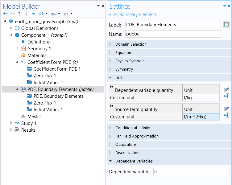
The Units settings for the PDE, Boundary Elements interface.
After this step we can change the name of the dependent variable to V, as shown in the figure below.
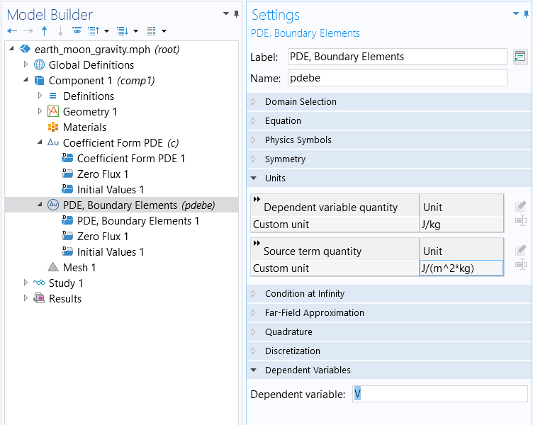
The Dependent variable settings for the PDE, Boundary Elements interface.
It is a feature in COMSOL Multiphysics® that by using the same name of the dependent variable in both interfaces, we get a consistent coupling between the two PDEs on any common boundary. For this to be possible, the units need to be the same in the two interfaces.
Recall that our strategy is to define Poisson's equation using the Coefficient Form PDE interface inside of the Earth and Moon, modeled as spheres, and then define a PDE, Boundary Elements interface to represent the gravity field in the surrounding space. In the figure below, you can see what this now looks like in the model tree.
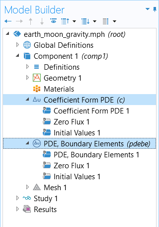
The mathematics interfaces used in the Earth–Moon gravity model.
We now need to specify an asymptotic value for the gravity potential, or the Condition at infinity. We will set this value to zero in the Settings window of the PDE, Boundary Elements interface. You can see these settings in the figure below.
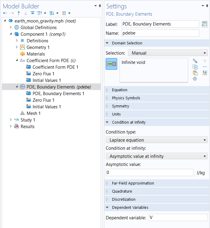
The Infinite void and Condition at infinity settings for the PDE, Boundary Elements interface.
If we use the analogy between Newtonian gravitation and electrostatics, we can view this asymptotic condition as a "Ground" boundary condition at a sphere very far away from the Earth–Moon system. In this way, we do not need to specify any actual boundary conditions for the Coefficient Form PDE interface. Instead, this Condition at infinity is propagating — from the Infinite void where the PDE, Boundary Elements interface is defined — inward via the coupling of the boundaries between the void and the two domains for the spheres. Again, the coupling is simply defined by assigning the same name of the dependent variable to the two equation interfaces.
With respect to the finite element mesh used in the spheres, a fixed element size of 500 km is used for the Earth, as shown in the figure below, and 200 km is used for the Moon. This is accomplished by setting the same value for the maximum and minimum element size. Inside of the spheres there will be tetrahedral finite elements. The boundary element mesh will consist of the triangular mesh at the surface of the spheres, adjacent to the Infinite void domain.
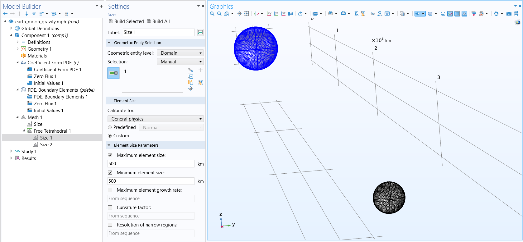 The COMSOL Multiphysics UI showing the Model Builder; the Mesh 1, Size 1 settings; and the Earth and Moon models in the Graphics window.
The settings for the finite element mesh of the Earth model.
Now, we can select Compute to solve the PDE system. The computation time is a few minutes.
The Results
We can plot the magnitude of the surface gravity,

corresponding to the expression sqrt(Vx^2+Vy^2+Vz^2), on the two planetary bodies, as shown in the figure below. You can type a mathematical expression like this one in the text fields for the expression to be visualized.
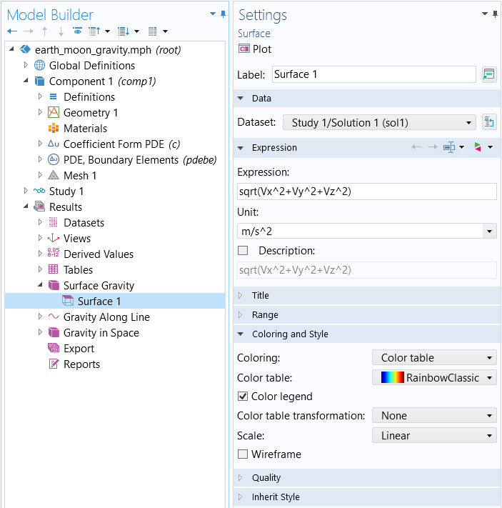
The expression used in a surface plot to visualize the magnitude of the surface gravity.
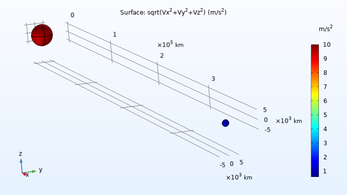
A Surface plot displaying the magnitude of surface gravity on the two planetary bodies.
Using a mouse, we can click on the surface of each sphere and read off the values 9.81 for the Earth and 1.62 for the Moon, which matches the expected values within less than a percent.
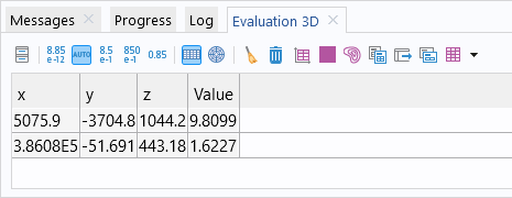
The table displaying the surface gravity, generated after clicking on the surface of each sphere in the results plot.
We can plot the magnitude of the gravity along a centerline in the space between the Earth and the Moon by plotting the variable pdebe.normgrad_u, a built-in variable used to efficiently compute the magnitude of the gravity vector field coming from the boundary element method solution. This gives us the plot shown below.
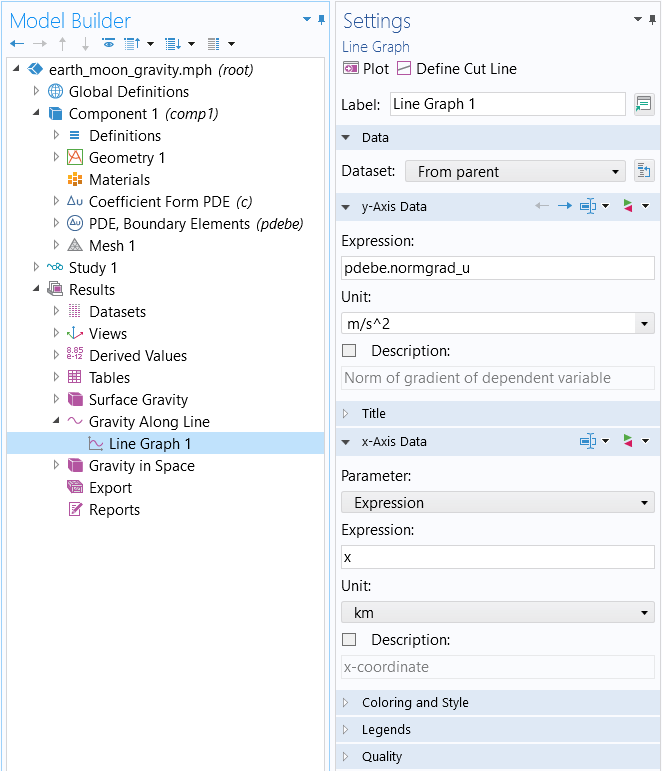
The settings for the plot where the built-in variable is used in the expression field.
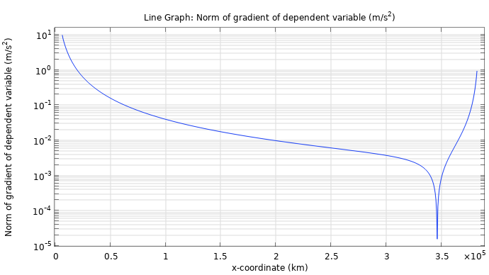
The gravity on a line between the Earth and the Moon using logarithmic scaling.
We can see a minimum at about 345,000 km. Note, however, that this does not correspond to one of the so-called Lagrange points. To compute the location of the Lagrange points, we would need to include the counteracting acceleration effects of a rotating frame due to orbital motion. Note that the Grid data settings were increased to produce this plot, as shown in the figure below. The Grid dataset adds volumetric grid cells so that boundary element quantities can be visualized and evaluated in void domains.
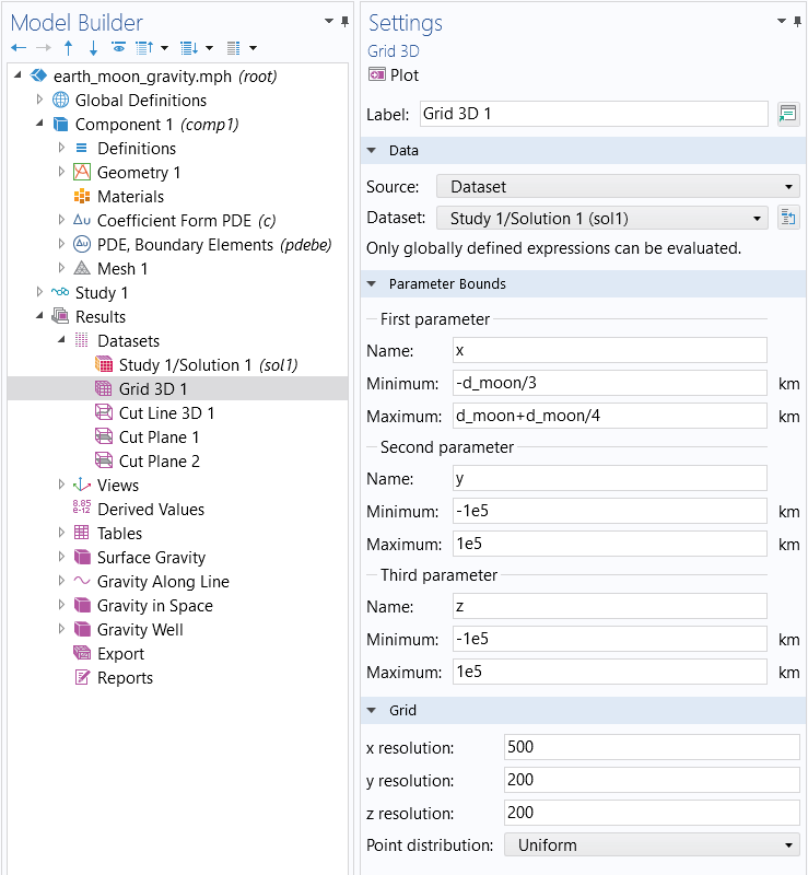
The settings for the Grid 3D dataset.
We can also visualize the gravitational field using colors, arrows, and contour lines, as shown in the figure below.
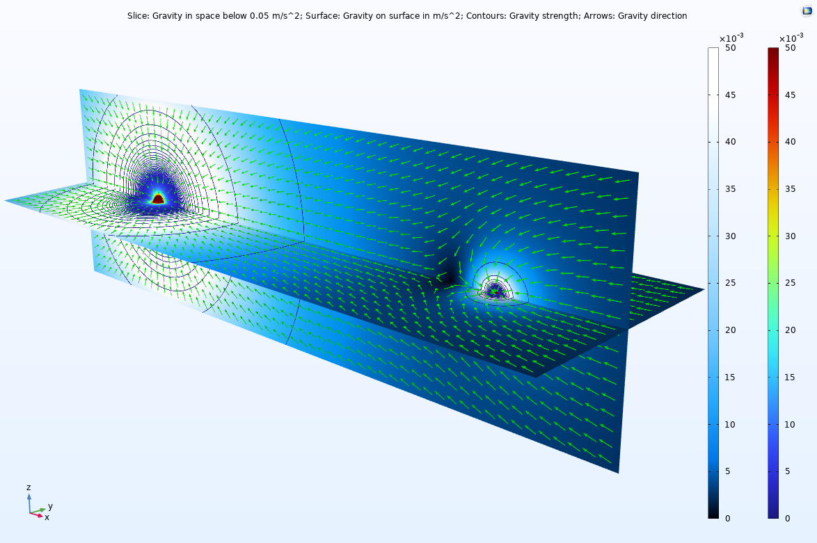 A slice plot of the Earth–Moon system compared to a blue color scale and Rainbow color scale with green arrows indicating the gravity direction.
In this visualization of the Earth–Moon system, the slice plot shows the gravity in space for values below 0.05 m/s2. The surface plots shows the gravity on the surfaces, the contours show the gravity strength, and the arrows show the direction of the gravitational field.
From this plot we can, for example, see that the Earth's gravity dominates a large area also close to the Moon. Only when we come fairly close to the Moon does the Moon's gravity take over.
As a final plot, we can create a "gravity well" plot by using a deformation modification of a cut plane plot, as shown in the figure below.
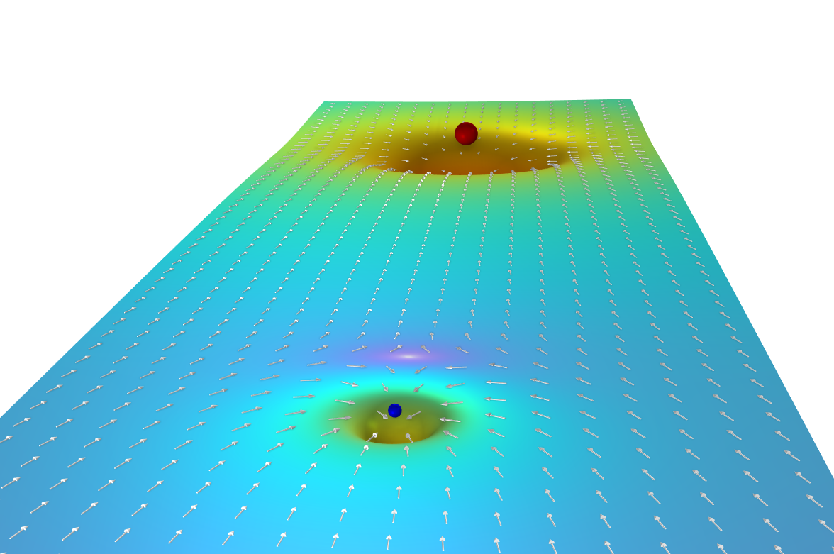
A gravity well plot of the Earth–Moon system.
The Inverse-Square Law
Since the PDE for gravitation might not be familiar, let us investigate how this relates to the more familiar inverse-square law for the gravitational force. The inverse-square law is actually encoded in Poisson's equation. To see this, consider a point source  having mass
  , located at the origin and the corresponding "point density"
  :
:

For the mathematically inclined reader, this equation is meaningful only in the weak sense.
The analytical solution to this equation is:

where  is the distance from the point source (origin).
We get the inverse-square law by taking the gradient in spherical coordinates:

where  is a unit vector pointing outward in the radial direction.
For more information on spherical coordinates, see this Wikipedia page.
We get the force  on a particle in this gravity field, having mass
  , by the relationship

which gives us the inverse square law:

Built-in Interfaces Based on the Boundary Element Method
For more information on using the built-in physics interfaces that are based on the boundary element method, please see the following blog posts:
- Acoustics: "How to Use the Boundary Element Method in Acoustics Modeling"
- Corrosion: "The Boundary Element Method Simplifies Corrosion Simulation"
- Magnetostatics: "Validating the Use of Boundary Elements for Magnetostatics Modeling"
- Electrostatics: "How to Create Electrostatics Models with Wires, Surfaces, and Solids"
Further Learning
The model used throughout this article is available for download. You can open and explore the model files to see exactly how the Laplace and Poisson's equations for the gravitational field of the Earth–Moon system were solved. In another Learning Center article we will examine the Coefficient Form PDE more.
Envoyer des commentaires sur cette page ou contacter le support ici.