Guidance for Solving Linear Stationary Models
A linear finite element model is one in which the material properties, loads, boundary conditions, and other model inputs are constant with respect to the solution. For the model to be considered linear, the governing partial differential equations themselves must also be linear. For a well-posed linear stationary model, the solver only needs to solve one large system of linear equations. If such a model does not solve, the cause is usually an issue with the model setup, constraints, material data, mesh, numerical conditioning, available memory, or solver configuration. Here, we will go over these potential issues and provide strategies for addressing them.
Background
While some of the guidance here can be applied generally in COMSOL Multiphysics®, much of it applies specifically to linear models that use a stationary solver. If you are unsure whether your problem is linear and stationary, first expand the branches under the Study node in the model tree to see if a Stationary Solver has been used. The Stationary Solver is used for both Stationary (time-invariant) and Frequency Domain (time-harmonic) study types. Next, near the top of the Log in the settings of the Stationary Solver node, check whether the software has reported that a linear or nonlinear solver was used (line highlighted in blue in the screenshot below).
Be aware that many multiphysics problems are nonlinear, especially when material properties, loads, boundary conditions, or couplings depend on the solution. If your model is nonlinear and you need help with solving, see our resource on Improving Convergence of Nonlinear Stationary Models.
 The Model Builder window with the Stationary Solver node selected and the respective settings open next to it in a panel.
The Stationary Solver log is opened to confirm that a model is linear and stationary.
The Model Builder window with the Stationary Solver node selected and the respective settings open next to it in a panel.
The Stationary Solver log is opened to confirm that a model is linear and stationary.
Setting Up Linear Models
In COMSOL Multiphysics®, the modeling workflow is the sequence of steps you take to set up, build, and compute the solution to your model equations. Following this procedure provides a guided approach to developing your model and helps ensure that the setup is complete. Resolving the following key issues related to settings and parameters (listed in the order of the modeling workflow) is particularly important when modeling linear stationary problems.
Insufficient Constraints and Boundary Conditions
To ensure that the solution for the dependent variables of a linear stationary model is unique, the constraints and boundary conditions must be sufficiently defined.
For example, in a model like the following — which uses the Solid Mechanics interface, where the software solves for the displacement in a solid — applying two opposite and equal Boundary Load conditions on a part is not sufficient to define the displacement. Even if the forces on a part are opposite and equal, this does not provide enough information to determine where the part is in space. To do so, you must add another condition, such as a Fixed Constraint boundary condition, which constrains the free rigid body displacements and rotations.
 A slender rectangular gray block with red arrows pointing outward from both the top surface and the bottom surface.
 An error window containing several lines of text indicating why the solver failed to to find a solution, noting the feature in the model tree where the issue is present.
In this example, we can add a Fixed Constraint boundary condition to the bottom boundary of the model. This condition fixes the boundary in place, similarly to how the model would be held in a tensile tester. The model is then fully constrained and can be solved.
You can find more information on various strategies for modeling parts without constraints in structural analyses in this blog post.
 A slender rectangular gray block with red arrows pointing outward from both the top and bottom surfaces, with the bottom surface colored in blue.
 A slender rectangular rainbow-colored block with red arrows pointing outward from the top surface and the bottom surface.
Undefined Material Properties
If any of a material's required properties is undefined, the software will generate an error at runtime and a red × will appear on the Materials node and the child node corresponding to the material. The properties required to compute the model are indicated in the settings of each Material node. In the Material Contents section, a blue checkbox indicates a required property is defined, and a red stop sign indicates a required property is missing.
 The Model Builder window with the Structural Steel material node selected, the respective Settings window, and the geometry assigned to the material colored in blue in the Graphics window.
The red × icons on the Materials and Structural Steel nodes warn that the material is not fully defined. In the settings of the Structural Steel node, the red stop sign indicates that the density value is missing.
The Model Builder window with the Structural Steel material node selected, the respective Settings window, and the geometry assigned to the material colored in blue in the Graphics window.
The red × icons on the Materials and Structural Steel nodes warn that the material is not fully defined. In the settings of the Structural Steel node, the red stop sign indicates that the density value is missing.
Incorrect Material Properties
It is also important to confirm that material properties have been defined correctly. Incorrect material properties can result in incorrect solutions or runtime errors (typically Singular Matrix errors) if the entered material properties are incompatible values.
For example, in an isotropic linear elastic material, setting Poisson’s ratio exactly to 0.5 represents the incompressible limit and can result in numerical instability with the standard formulation or a singular stiffness matrix. To avoid these issues, use a physically appropriate value below 0.5, or use a formulation intended for incompressible or nearly incompressible materials. The image above shows an example where Poisson’s ratio is entered incorrectly.
 An Error window containing several lines of text indicating the feature in the model tree where the issue is present and that the solver failed because it could not evaluate a variable.
Undefined Variables
Similarly to undefined material properties, an undefined variable will produce a runtime error that provides information about the variable name and where it is being used. Automatic syntax highlighting can help you identify undefined variables as you enter expressions. It is best practice to resolve undefined variables as soon as they are identified, before attempting to solve the model.
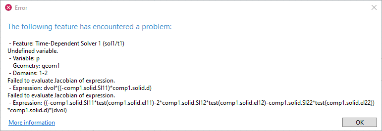 An Error window containing several lines of text indicating the feature in the model tree where the issue is present and that the solver failed due to an undefined variable.
Solver Configuration
Once you have confirmed that the model is sufficiently constrained and that all materials are correctly defined, check the solver settings. If you are in doubt, start with the default solver settings by resetting the solver to its defaults.
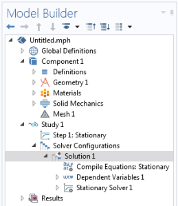
Resetting the Solver
Each physics interface, or combination of physics interfaces, in your model has different default solvers. However, if a lower-level change has been made manually to the solver settings, the software will not automatically use the default solver. The solver settings are stored at Study > Solver Configurations > Solution. If these settings have been manually changed, you will see a small star symbol on the Solution feature, as shown in the screenshot below. If you see this, right-click on the Solution feature and select Reset Solver to Default. Alternatively, delete and re-create the study. You can learn more about the direct and iterative solvers through this resource: "Understanding the Fully Coupled vs. Segregated Approach and Direct vs. Linear Solvers".
 A cropped section of the model tree with the Solution node selected.
Out of Memory
If a model is very large and your computer lacks sufficient memory, you may get an error message regarding memory when attempting to solve. This is not an issue with the solvability of the model, but with the computational resources available. Refer to our resource that addresses the Error: "Out of memory" dialog for more information on this error.
If adding more memory or using a different computer is not an option, there are alternatives that may allow your simulation to run. These include starting with as coarse a mesh as possible and refining more gradually. If the model is otherwise well posed, a coarser mesh can reduce memory requirements and may help determine whether the failure is due to problem size rather than model setup. Mesh coarsening will not fix missing constraints, undefined variables, invalid material properties, or a singular formulation. See "Performing a Mesh Refinement Study" for more information on automating this approach.
 An error window containing several lines of text indicating why the solver failed, due to running out of memory, and the feature in the model tree where the issue is present.
Extremely Ill-Conditioned Problems
Some models are inherently numerically ill-conditioned. A numerically ill-conditioned model has a system matrix that is nearly singular, making it difficult to solve on a finite-precision computer. This can arise from extreme variations in material properties or from geometry with a high aspect ratio. If this is true for your model, there are approaches that can be used to overcome these obstacles. A few examples of ill-conditioned problems and techniques for resolving them are shown below. You can learn more about nearly singular matrices by referencing the following resource here.
Materials
In an electric currents problem, you may want to model a system of materials that includes a good conductor, such as copper, with an electrical conductivity of approximately  , and an insulating material, such as glass, which can have an electrical conductivity of approximately
  . Such a large difference in material properties can be challenging.
In such cases, see whether one material or the other can be omitted from the analysis completely. In this case, it would likely be reasonable to treat the insulating material as a perfect insulator, omit it from the analysis, and use the Electric Insulation boundary condition instead of modeling those domains.
 A cropped section of the model tree with the Electric Insulation node selected.
Geometry
The conditions on the geometric aspect ratio are relatively strict. As a rough rule of thumb, once the aspect ratio between the largest characteristic dimension and the smallest characteristic dimension approaches  , you may start to run into issues and should look for alternative ways of posing the problem, especially for a 3D model.
An example would be a linear static structural model of an aluminum beverage can. If this were solved using the Solid Mechanics interface the thin walls of the container would need to be explicitly modeled, but the wall thickness is much smaller than the overall can dimensions. Such a case would be better addressed with the Shell interface, which is specially formulated for handling thin-walled structural parts.
In many physics areas, alternative physics formulations are available for solving cases where the geometry has an extreme aspect ratio. These can be used alone or in combination with other interfaces. Ideally, these formulations should be used instead of explicitly modeling high-aspect-ratio parts of geometries.
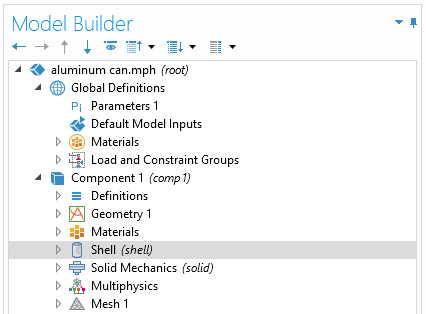 A cropped section of the model tree with the Shell node selected.
Meshing
In some cases an extremely poor-quality mesh can lead to an ill-conditioned problem. This issue often arises in combination with, and as a consequence of, geometries that have extreme aspect ratios. Using a manually defined mesh is one way to avoid elements with extreme aspect ratios. If you are building a user-defined mesh, you can reference the course "Using Swept Meshes for Model Geometries" and more specifically the section on use cases for swept meshes to learn more about how they can be applied to more complex geometric elements, such as those with extreme aspect ratios.
Performing a mesh refinement study can help in a variety of situations, including ill-conditioned problems, due to a poor mesh as well as errors due to insufficient memory, as mentioned previously. To learn more about how to implement a mesh refinement study, see "Performing a Mesh Refinement Study".
Solvers
For ill-conditioned problems, a direct solver can be more robust, but may require substantially more memory. The default solver for many 3D models is an iterative solver, which is more sensitive to ill-conditioned problems. If the default iterative solver is not converging, try switching to a direct solver, as described in "Understanding the Fully Coupled vs. Segregated approach and Direct vs. Linear solvers". A direct solver will not fix a singular or physically ill-posed model.
 A cropped section of the model tree with the Fully Coupled node selected.
The iterative solver being used within the Fully Coupled feature.
A cropped section of the model tree with the Fully Coupled node selected.
The iterative solver being used within the Fully Coupled feature.
Envoyer des commentaires sur cette page ou contacter le support ici.