Centre d'apprentissage

Using an External Excitation to Analyze an Optical Resonant Structure

When modeling an optical resonant structure using the COMSOL Multiphysics^® software and its add-on Wave Optics Module, there are multiple approaches you can use to analyze the structure. This includes using an eigenfrequency study to directly compute the optical properties of a resonator. You can also use an external excitation. Using an external excitation enables you to calculate the transmitted and reflected fields of the resonant structure and then determine optical properties such as the quality factor and the finesse. Here, we provide an introduction on how to implement this approach.

Tutorial: Using an External Excitation to Analyze an Optical Resonant Structure

Follow along in the software as we quickly build an example model of a Fabry–Pérot etalon to present the basic workflow for using an external excitation to analyze the structure. The parameters for the model are attached to this article.

The general procedure for applying this approach is outlined below. Important aspects of each step are highlighted following the tutorial.

1. Create the geometry and assign the material properties.
2. Define the transparent boundaries and external excitation.
3. Perform a wavelength sweep.

Defining Transparent Boundaries and an Excitation

Transparent boundaries are critical in simulations for preventing reflections from the edges of the model, which can distort results. In an optical simulation, for example, these boundaries ensure that light exiting the modeled region does not reenter it, mimicking an infinite space. Additionally, defining an excitation, such as a paraxial-approximate Gaussian beam, is essential for accurately simulating real-world scenarios.

The Scattering Boundary Condition feature is a simple way to make an outer boundary of a model transparent. It can also be used to define an excitation. There are different options available under the Incident field setting, but for our example of modeling an etalon, we use a paraxial-approximate Gaussian beam as the light source.

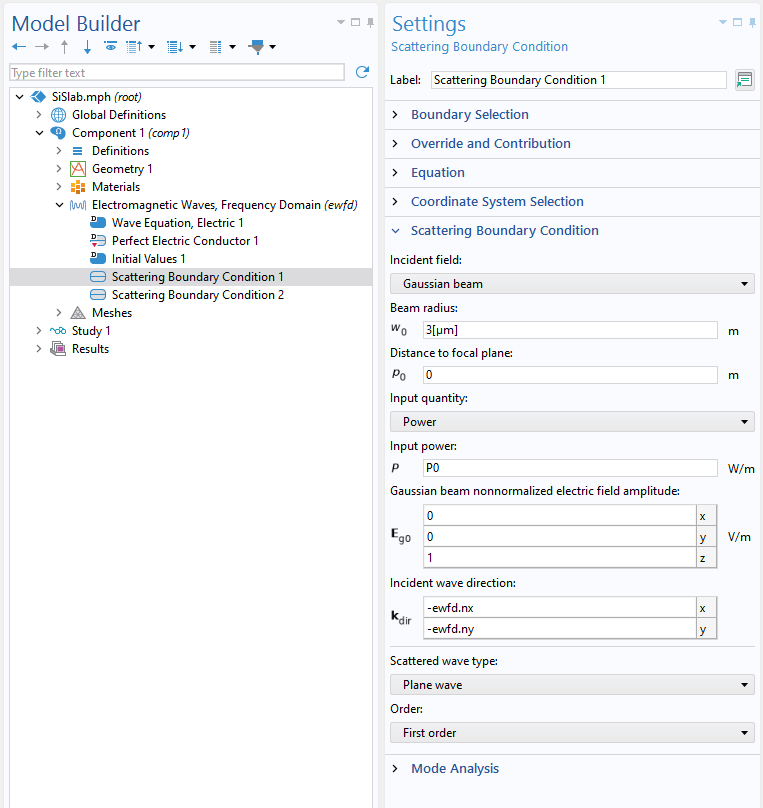The Model Builder with the Scattering Boundary Condition 1 node selected and the corresponding Settings window open, which includes multiple menus and text input fields with Gaussian beam selected for the incident field.

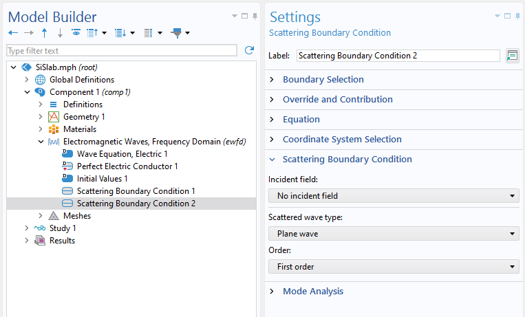The Model Builder with the Scattering Boundary Condition 2 node selected and the corresponding Settings window open, which includes multiple menus with No incident field selected for the incident field.

The Scattering Boundary Condition feature is used to define the light source (left) and the transparent boundaries (right).

Analyzing the Reflected and Transmitted Signal

The transmitted and reflected signal — in particular, the power — can give us information about the resonant behavior and thus needs to be evaluated on both the input and output sides of the structure. This evaluation can be done manually using variables and an Integration operator on the input and output sides. To get the reflected signal, we can subtract the incident field from the total field. The absorptivity can then be computed by integrating over the losses.

Here, is the characteristic impedance of vacuum and is the input power. In COMSOL Multiphysics^® version 6.4, a convenient way to compute these properties was introduced through the addition of predefined global variables for each Scattering Boundary Condition. The variables, ewfd.sctr1.etaOut and ewfd.sctr2.etaOut, represent the outcoupling efficiency on the input and output sides, respectively.

Performing a Wavelength Sweep to Analyze the Resonant Behavior

Reflection, transmission, and absorption signals all show a modulation characteristic for the etalon resonant structure. A wavelength sweep is performed using the Wavelength Domain study and specifying a range of values for the wavelength in the settings. To visualize the results for the optical properties, a 1D plot is created. The transmission profile gives us information about the resonant behavior of the structure. The broad peaks are a sign of the bad optical quality of the resonator, which is caused by the high losses that result from the low reflectivity of the uncoated silicon slab. From the profile, you can derive optical properties like the optical quality factor or the finesse of the resonator.

The profiles for the transmittance, reflectance, and absorptance properties of an etalon modeled in the software.

Graph Marker subnodes are used to automatically add markers to a plot at the maximum values, in addition to extracting the location and values of the maxima into a table.

Benefits and Challenges of this Approach

Using an external excitation to probe the resonant structure can be quite convenient as it is similar to how such a device would be studied in the lab, making it easy to compare to measured data. Applying this approach to resonators with a high optical quality factor can be challenging as the resonance can become very narrow, requiring a high resolution in the wavelength sweep to accurately capture the peak. Performing a discrete wavelength sweep can be time consuming, especially if you don’t exactly know where the resonance is, and you need multiple datapoints of the resonance for analysis.

In such cases, the Adaptive Frequency Sweep study type can significantly reduce computation time by dynamically adjusting the frequency step size based on the response of the system. This method focuses on regions with rapid changes, such as near resonances, while using larger steps in areas with less variation, thereby optimizing the process. In the Application Libraries, tutorial models that demonstrate the use of this study can be found by entering @study:frawe in the search field. Other ways to search for models are discussed extensively in the article "How to Search for Relevant Modeling Examples".

Further Learning

• Tutorial models:
  • Model a simple optical resonant structure and compute the Q factor: Fabry–Perot Cavity
  • Perform a frequency sweep to evaluate the Q factor: RF Coil
• COMSOL documentation:
  • Coupling Between Sources and Destinations
• Blog posts:
  • "Methods That Accelerate the Modeling of Bandpass Filter Type Devices"
  • "Understanding the Paraxial Gaussian Beam Formula"