Centre d'apprentissage

Modeling Acoustic Ray Tracing: Release from Boundary

---

We now look into the other surface ray source option using the Release from Boundary feature. This method is useful when the surface intensity data comes from measurements or simulations performed in a separate model. In such cases, the intensity data is imported into the ray acoustics model via interpolation functions, similar to the approach used  for the Source with Directivity ray release option. However, for comparison purposes, we will demonstrate this option within the same model we just created for the Release from Pressure Field release option.

Keeping all previous settings intact, we proceed to add a Release from Boundary node to the Ray Acoustics interface and configure it as follows:

1. First, in the Initial Position section, select Density for Initial position, enter Nrays in the Number of rays per release input field, and keep the default values for the other inputs. These settings ensure that rays are evenly distributed among the mesh elements and that each ray is assigned a unique position.

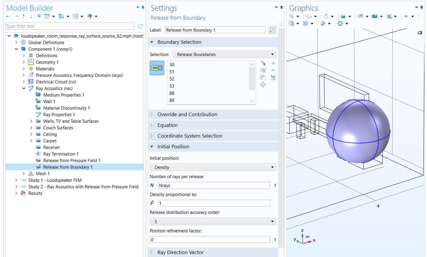A blue sphere surrounds the wireframe of the speaker with the settings for the release from boundary node open. Initial ray position setup.

2. Then, in the Ray Direction Vector section, use the normalized intensity vector (acpr.Ix/acpr.I_mag, acpr.Iy/acpr.I_mag, acpr.Iz/acpr.I_mag) to define the ray direction vector, where acpr.Ix, acpr.Iy, acpr.Iz, and acpr.I_mag are the x, y, z components of the acoustic intensity and its magnitude, respectively, calculated in the source model. The concept is that the rays are emitted from the release surface in the direction of the acoustic intensity. Note that the expressions are enclosed in the bndenv( ) operator, which evaluates them at the coordinates of each ray at the boundary. This ensures that the FEM solution is correctly mapped onto the rays.

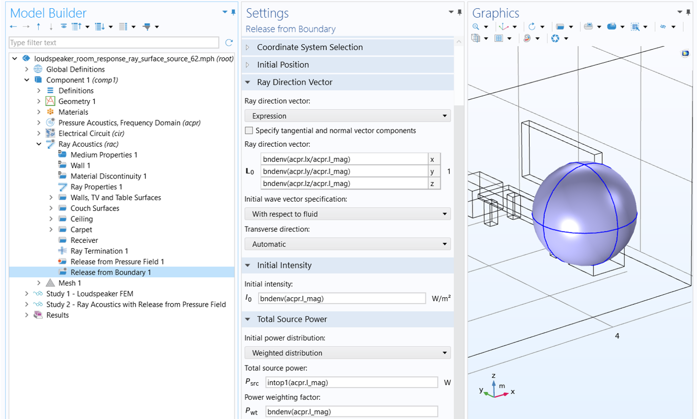The ray direction vector, initial intensity, and total source power are applied to a blue sphere surrounding a wireframe speaker. Ray direction, initial intensity, and initial power setup.

3. Finally, specify rays' initial intensity and power based on the intensity magnitude (see the image above). In the Initial Intensity section, enter bndenv(acpr.I_mag) for Initial intensity. In the Total Source Power section, select Weighted distribution for Initial power distribution, enter intop1(acpr.I_mag) for Total source power and bndenv(acpr.I_mag) for Power weighting factor. The intop1( ) operator, defined under Component 1 > Definitions, integrates the enclosed expression over the release boundaries. These settings ensure that each ray is released with the magnitude of the local intensity and that the total radiation power and its distribution are correctly mapped from the FEM solution to the ray acoustics model.

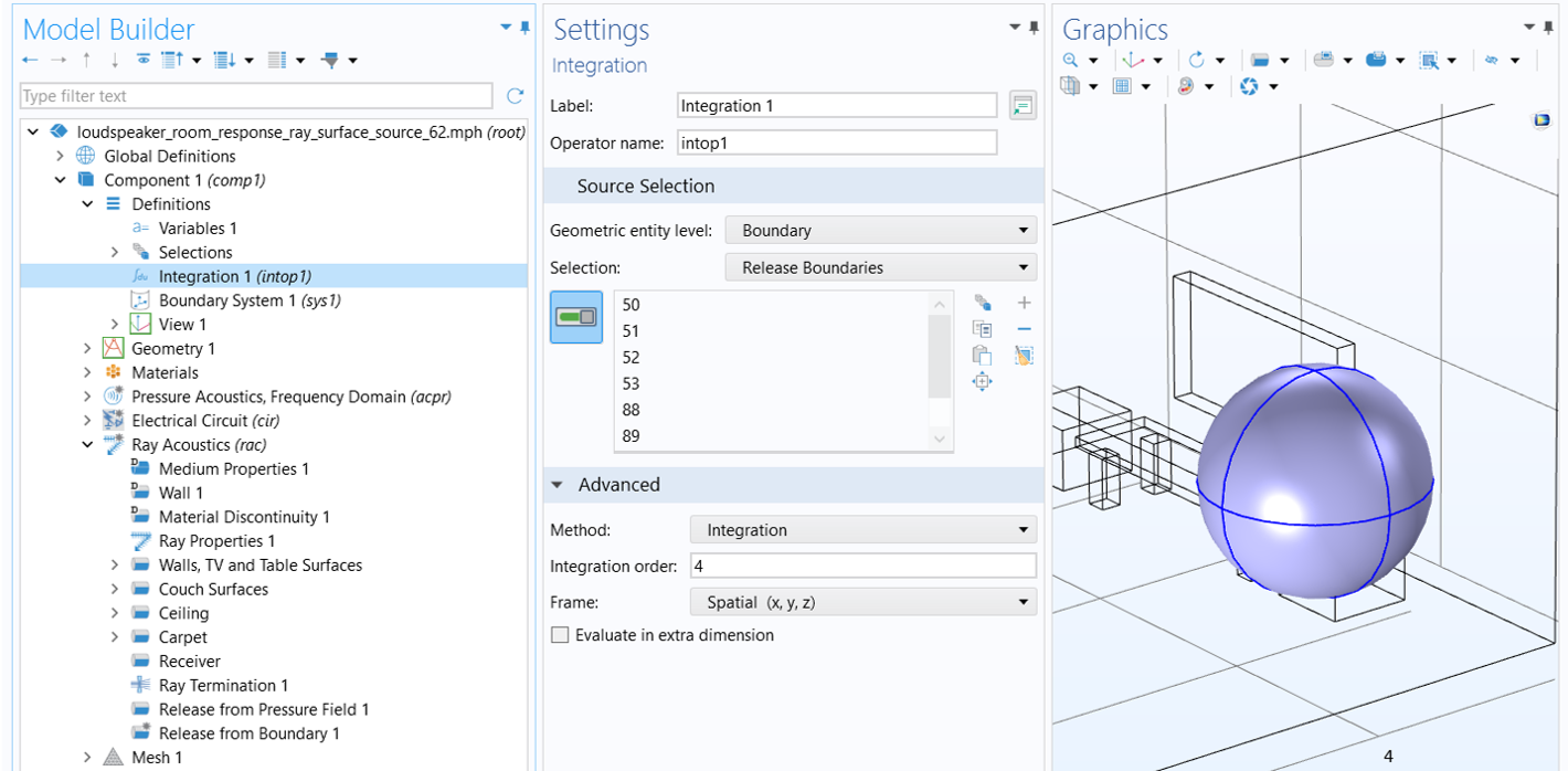The boundaries of a blue sphere on the right are selected in the integration settings window on the left. The intop1( ) operator is defined to calculate the integration of the enclosed expression over the release boundaries.

Add a new Ray Tracing study and a Parametric Sweep node to it to solve for this release method. Make sure that the Release from Pressure Field node is disabled for this study in the  Physics and Variables Selection section of the Ray Tracing study settings, as shown below. To do this, enable  Modify model configuration for study step (check the box), then click the Release from Pressure Field node and disable it using the Disable button in the toolbar below. This ensures that only the Release from Boundary node is used for releasing rays. All other study settings should remain the same as those used in Study 2 for the Release from Pressure Field option. Please note that if you want to resolve Study 2 using the Release from Pressure Field option, you'll need to disable the Release from Boundary node in the same manner to ensure the correct release method is used.

The figure below compares the frequency spectrum of the impulse response obtained using this release option (green curve) with that from the Release from Pressure Field option (blue curve). The two approaches yield nearly identical results, as expected, since both are based on the intensity vector on the release surface derived from the source model.

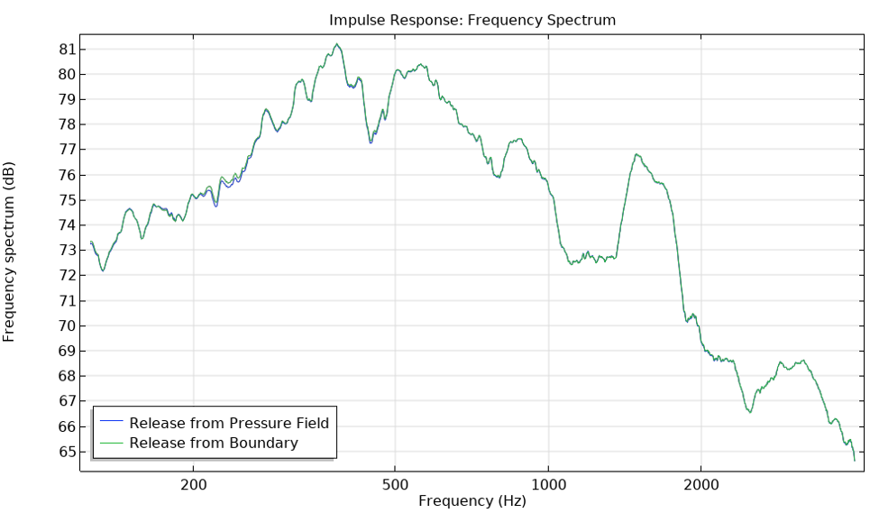A line graph comparing the frequency spectrum using the release from pressure field (blue) and release from boundary (green) at various frequencies. Comparison of impulse response obtained using the two surface release options.

Comparison of Results Using Different Methods

We now compare the solutions obtained using point and surface ray release methods with the results from the full-wave FEM analysis conducted in Part 1. The figure below illustrates this comparison by showing the frequency spectrum of the impulse response from the two ray-tracing approaches—Release from Exterior Field Calculation (point ray source) and Release from Pressure Field (surface ray source)—alongside the frequency response from the full-wave FEM model. Note that no smoothing is applied to the FEM results, whereas a 1/3-octave moving average filter is applied to the ray-tracing results.

The curves exhibit the same overall behavior. They also indicate strong modal behavior in the room even above the estimated Schroeder frequency (approximately 281 Hz), in this case extending to the upper limit of the frequency range resolved in the FEM model. Therefore, it is recommended to use the full-wave method up to the highest frequency your computer can handle, and to switch to ray tracing only beyond that point. 

A noticeable level difference is observed between the two ray acoustics results (the green and red curves), attributed to several distinctions in the underlying source descriptions. First, the point ray source is extracted from a source model that assumes the speaker radiates into open space, whereas the surface ray source is computed while accounting for scattering from nearby structures. As a result, the acoustic energy is distributed differently in the two cases. Second, the temporal distribution of energy arriving at the receiver differs between the two source models. As noted earlier, in the surface ray source case all rays are released simultaneously, and the time delay between the point ray source and the surface ray source is not taken into account. 

A line graph comparing the sound pressure levels for the full-wave FEM (blue), release from exterior field calculation (green) and release from pressure field (red) at various frequencies. Comparison of sound pressure levels measured at the receiver using different methods.

The FEM solution at low frequencies can now be combined with the ray acoustics solution at high frequencies to produce a broadband frequency response and impulse response. This approach is demonstrated in two tutorials—Modeling Room Acoustics Using Hybrid Pressure Acoustics and Ray-Tracing Methods and Car Cabin Acoustics – Broadband Impulse Response—and is explained in detail in the blog post titled Modeling Room Acoustics Using a Hybrid Approach.