

The most fundamental material model for structural mechanics analysis is the linear elastic model. Trivial as it may sound, there are some important details that may not be obvious at first glance. In this blog post, we will dive deeper into the theory and application of this material model and give an overview of isotropy and anisotropy, allowable values for material data, incompressibility, and interaction with geometric nonlinearity.
Isotropic Linear Elasticity
In the vast majority of simulations involving linear elastic materials, we are dealing with an isotropic material that does not have any directional sensitivity. To describe such a material, only two independent material parameters are required. There are many possible ways to select these parameters, but some of them are more popular than others.
Young’s Modulus, Shear Modulus, and Poisson’s Ratio
Young’s modulus, shear modulus, and Poisson’s ratio are the parameters most commonly found in tables of material data. They are not independent, since the shear modulus, G, can be computed from Young’s modulus, E, and Poisson’s ratio, \nu, as
Young’s modulus can be directly measured in a uniaxial tensile test, while the shear modulus can be measured in, for example, a pure torsion test.
In the uniaxial test, Poisson’s ratio determines how much the material will shrink (or possibly expand) in the transverse direction. The allowable range is -1 <\nu< 0.5, where positive values indicate that the material shrinks in the thickness direction while being pulled. There are a few materials, called Auxetics, which have a negative Poisson’s ratio. A cork in a wine bottle has a Poisson’s ratio close to zero, so that its diameter is insensitive to whether it is pulled or pushed.
For many metals and alloys, \nu \approx1/3, and the shear modulus is then about 40% of Young’s modulus.
Given the possible values of \nu, the possible ratios between the shear modulus and Young’s modulus are
When \nu approaches 0.5, the material becomes incompressible. Such materials pose specific problems in an analysis, as we will discuss.
Bulk Modulus
The bulk modulus, K, measures the change in volume for a given uniform pressure. Expressed in E and \nu, it can be written as:
When \nu= 1/3, the value of the bulk modulus equals the value of Young’s modulus, but for an incompressible material (\nu \to0.5), K tends to infinity.
The bulk modulus is usually specified together with the shear modulus. These two quantities are, in a sense, the most physically independent choices of parameters. The volume change is only controlled by the bulk modulus and the distortion is only controlled by the shear modulus.
Lamé Constants
The Lamé constants \mu and \lambda are mostly seen in more mathematical treatises of elasticity. The full 3D constitutive relation between the stress tensor \boldsymbol \sigma and the strain tensor \boldsymbol \varepsilon can be conveniently written in terms of the Lamé constants:
The constant \mu is simply the shear modulus, while \lambda can be written as
A full table of conversions between the various elastic parameters can be found here.
Incompressibility in Linear Elastic Materials
Some materials, like rubber, are almost incompressible. Mathematically, a fully incompressible material differs fundamentally from a compressible material. Since there is no volume change, it is not possible to determine the mean stress from it. The state equation for the mean stress (pressure), p, as function of volume change, \Delta V, as
will no longer exist, and must instead be replaced by a constraint stating that
Another way of looking at incompressibility is to note that the term (1-2\nu) appears in the denominator of the constitutive equations, so that a division by zero would occur if \nu= 0.5. Is it then a good idea to model an incompressible material approximately by setting \nu= 0.499?
It can be done, but in this case, a standard displacement based finite element formulation may give undesirable results. This is caused by a phenomenon called locking. Effects include:
- Overly stiff models.
- Checkerboard stress patterns.
- Errors or warnings from the equation solver because of ill-conditioning.
The remedy is to use a mixed formulation where the pressure or volumetric strain is introduced as an extra degree of freedom. In COMSOL Multiphysics, you enable a mixed formulation by selecting one of the methods available in the Use mixed formulation checkbox in the settings for the material model
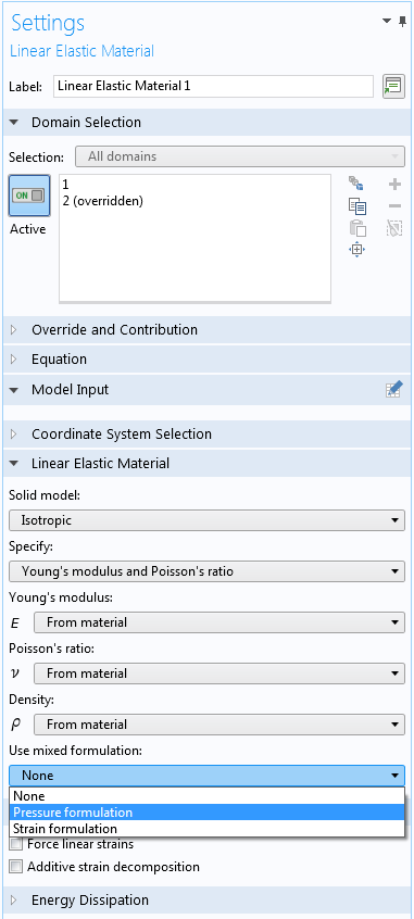
Part of the settings for a linear elastic material with mixed formulation enabled.
When Poisson’s ratio is larger than about 0.45, or equivalently, the bulk modulus is more than one order of magnitude larger than the shear modulus, it is advisable to use a mixed formulation. An example of the effect is shown in the figure below.
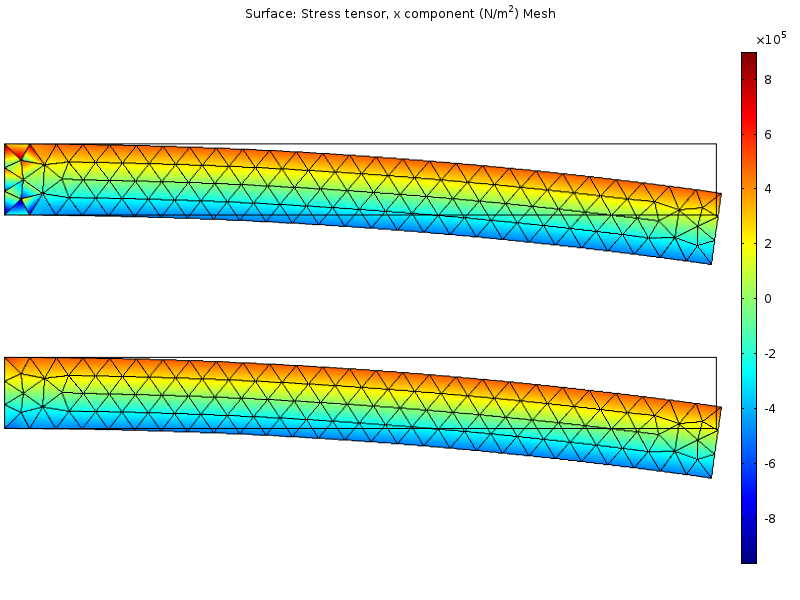
Stress distribution in a simple plane strain model, \nu = 0.499. The top image shows a standard displacement based formulation, while the bottom image shows a mixed formulation.
In the solution with only displacement degrees of freedom, the stress pattern shows distortions at the left end where there is a constraint. These distortions are almost completely removed by using a mixed formulation.
Orthotropy and Anisotropy
In general cases of linear elastic materials, the material properties have a directional sensitivity. The most general case is called anisotropic, which means all six stress components can depend on all six strain components. This requires 21 material parameters. Clearly, it is a demanding task to obtain all of this data. If the stress, \boldsymbol \sigma, and strain, \boldsymbol \varepsilon, are treated as vectors, they are related by the constitutive 6-by-6 symmetric matrix \mathbf D through
Fortunately, it is common that nonisotropic materials exhibit certain symmetries. In an orthotropic material, there are three orthogonal directions in which the shear action is decoupled from the axial action. That is, when the material is stretched along one of these principal directions, it will only contract in the two orthogonal directions, but not be sheared. A full description of an orthotropic material requires nine independent material parameters.
The constitutive relation of an orthotropic material is easier when written on compliance form, \boldsymbol \varepsilon= \mathbf C \boldsymbol \sigma:
\begin{bmatrix}
\tfrac{1}{E_{\rm X}} & -\tfrac{\nu_{\rm YX}}{E_{\rm Y}} & -\tfrac{\nu_{\rm ZX}}{E_{\rm Z}} & 0 & 0 & 0 \\
-\tfrac{\nu_{\rm XY}}{E_{\rm X}} & \tfrac{1}{E_{\rm Y}} & -\tfrac{\nu_{\rm ZY}}{E_{\rm Z}} & 0 & 0 & 0 \\
-\tfrac{\nu_{\rm XZ}}{E_{\rm X}} & -\tfrac{\nu_{\rm YZ}}{E_{\rm Y}} & \tfrac{1}{E_{\rm Z}} & 0 & 0 & 0 \\
0 & 0 & 0 & \tfrac{1}{G_{\rm YZ}} & 0 & 0 \\
0 & 0 & 0 & 0 & \tfrac{1}{G_{\rm ZX}} & 0 \\
0 & 0 & 0 & 0 & 0 & \tfrac{1}{G_{\rm XY}} \\
\end{bmatrix}
Since the compliance matrix must be symmetric, the twelve constants used are reduced to nine through three symmetry relations of the type
Note that \nu_{\rm YX} \neq \nu_{\rm XY}, so when dealing with orthotropic data, it is important to make sure that the intended Poisson’s ratio values are used. The notation may not be the same in all sources.
Anisotropy and orthotropy commonly occur in inhomogeneous materials. Often, the properties are not measured, but computed using a homogenization process upscaling from microscopic to macroscopic scale. A discussion about such homogenization — in quite another context – can be found in this blog post.
For nonisotropic materials, there are limitations to the possible values of the material parameters similar to those described for isotropic materials. It is difficult to immediately see these limitations, but there are two things to look out for:
- The constitutive matrix \mathbf D must be positive definite.
- For a general anisotropic material, the only option is to check if all of its eigenvalues are positive.
- For an orthotropic material, this is true if all six elastic moduli are positive and \nu_{\rm XY}\nu_{\rm YX}+\nu_{\rm YZ}\nu_{\rm ZY}+\nu_{\rm ZX}\nu_{\rm XZ}+\nu_{\rm YX}\nu_{\rm ZY}\nu_{\rm XZ}<1
- If the material has low compressibility, a mixed formulation must be used.
- It is possible to make an estimate of an effective bulk modulus and the values of the shear moduli.
- In cases of uncertainty, it is better to take the extra cost of the mixed formulation to avoid possible inaccuracies.
Geometric Nonlinearity
When working with geometrically nonlinear problems, the meaning of “linear elasticity” is really a matter of convention. The issue here is that there are several possible representations of stresses and strains. For a discussion about different stress and strain measures, see this previous blog post.
Since the primary stress and strain quantities in COMSOL Multiphysics are Second Piola-Kirchhoff stress and Green-Lagrange strain, the natural interpretation of linear elasticity is that these quantities are linearly related to each other. Such a material is sometimes called a St. Venant material.
Intuitively, one could expect that “linear elasticity” means that there is a linear relation between force and displacement in a simple tensile test. This will not be the case, since both stresses and strains depend on the deformation. To see this, consider a bar with a square cross section.
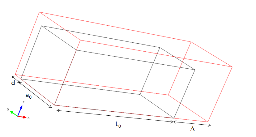
The bar subjected to uniform extension.
The original length of the bar is L_0 and the original cross-section area is A_0=a_0^2, where a_0 is the original edge of the cross section. Assume that the bar is extended at a distance \Delta so that the current length is L=L_0+\Delta=L_0(1+\xi).
Here, 1+\xi is the axial stretch and \xi can be interpreted as the engineering strain. The new length of the edge of the cross section is a=a_0+d=a_0(1+\eta), where \eta is the engineering strain in the transverse directions.
The force can be expressed as the Cauchy stress \sigma_x in the axial direction multiplied by the current cross-section area:
To use the linear elastic relation, the Cauchy stress \boldsymbol \sigma must be expressed as the Second Piola-Kirchoff stress \mathbf S. The transformation rule is
where \mathbf F is the deformation gradient tensor, and the volume scale is defined as J = det(\mathbf F). Without going into details, for a uniaxial case
Since for a St. Venant material in uniaxial extension, the axial stress is related to the axial strain as S_X = E \epsilon_X, we obtain
Given that the axial term of the Green-Lagrange strain tensor is defined as
the force versus displacement relation is then
The linear elastic material furbished with geometric nonlinearity actually implies a cubic relation between force and engineering strain (or force versus displacement, since \Delta =L_0\xi), as shown in the figure below.
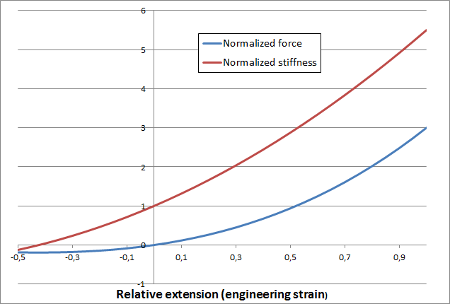
The uniaxial response of a linear elastic material under geometric nonlinearity.
As can be seen in the graph, the stiffness of the material approaches zero at the compression side, \xi = \sqrt{{1}/{3}}-1 \approx -0.42. In practice, this means that the simulation will fail at that strain level. It can be argued that there are no real materials that are linear at large strains, so this should not cause problems in practice. However, linear elastic materials are often used far outside the range of reasonable stresses for several reasons, such as:
- Often, you may want to do a quick “order of magnitude” check before introducing more sophisticated material models.
- There are singularities in the model that cause very high strains in a point.
- Read more about singularities here.
- In contact problems, the study is always geometrically nonlinear.
- Often, high compressive strains appear locally in the contact zone at some time during the analysis.
In all of these cases, the solver may fail to find a solution if the compressive strains are large. If you suspect this to be the case, it is a good idea to plot the smallest principal strain. If it is smaller than -0.3 or so, we can expect this kind of breakdown. The critical value in terms of the Green-Lagrange strain is found to be -1/3. When this becomes a problem, you should consider changing to a suitable hyperelastic material model.
Compression may not be the only problem. In the analysis above, Poisson’s ratio did not enter the equations. So what happens with the cross section?
By definition in the uniaxial case, the transverse strain is related to the axial strain by
When these strains are Green-Lagrange strains, this is a nonlinear relation stating that
Thus, there is a strong nonlinearity in the change of the cross section. Solving this quadratic equation gives the following relation between the engineering strains
The result is shown in the figure below.
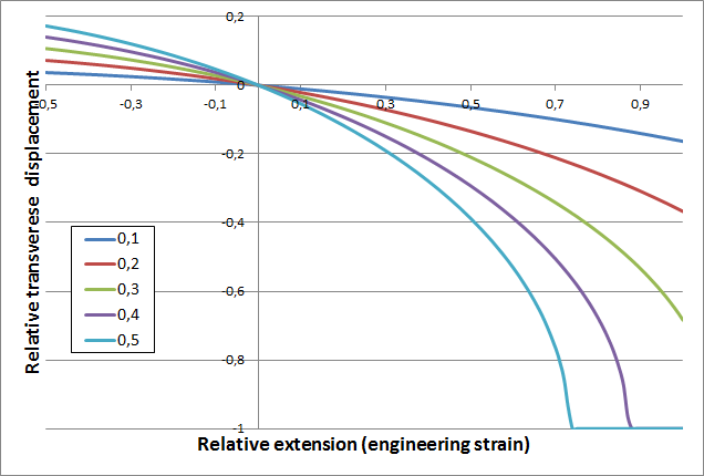
Transverse displacement as a function of the axial displacement for uniaxial tension of a St. Venant material. Five different values of Poisson’s ratio are shown.
As you can see, the cross section collapses quickly at large extensions for higher values of Poisson’s ratio.
If another choice of stress and strain representation had been made — for example, if the Cauchy stress were proportional to the logarithmic, or “true” strain — it would have resulted in quite a different response. Instead, such a material has a stiffness that decreases with elongation, where the force-displacement response does depend on the value of Poisson’s ratio. Still, both materials can correctly be called “linear elastic”, although the results computed with large strain elasticity can differ widely between two different simulation platforms.
Concluding Remarks on Linear Elastic Materials
We have illustrated some limits for the use of linear elastic materials. In particular, the possible pitfalls related to incompressibility and to the combination of linear elasticity with large strains have been highlighted.
If you are interested in reading more about material modeling in structural mechanics problems, check out these blog posts:
- Introducing Nonlinear Elastic Materials
- Obtaining Material Data for Structural Mechanics from Measurements
- Part 2: Obtaining Material Data for Structural Mechanics from Measurements
- Fitting Measured Data to Different Hyperelastic Material Models
- Yield Surfaces and Plastic Flow Rules in Geomechanics
- Computing Stiffness of Linear Elastic Structures: Part 1
- Computing Stiffness of Linear Elastic Structures: Part 2
Editors note: From version 5.4, the settings for mixed formulations look different, since more options were added.


Comments (6)
Casper Holst
April 6, 2016Thanks Henrik, for this blogpost.
Can you recommend some good literature for e.g. Geometric Nonlinearity, and where I can find some more about Cauchy and Piola-Kirchoff stresses
Henrik Sönnerlind
April 13, 2016Hi Casper,
Here are a couple of good online resources:
http://www.solidmechanics.org
http://www.continuummechanics.org
There are many good books, one example is
Holzapfel, G.; Nonlinear Solid Mechanics: A Continuum Approach for Engineering
Regards,
Henrik
SomtoChukwu Ufondu
April 23, 2018Hi Henrik,
I was wondering whether the relation for the compliance matrix for anisotropic materials should not instead be “nu_{yx}/E_y = nu_{xy}/E_x.”
Henrik Sönnerlind
April 24, 2018Hi SomtoChukwu,
Thanks for bringing this to our attention. The typo is fixed now.
Regards,
Henrik
MOHAMMAD ASIF RAJA
August 5, 2020How can one extract data to plot the results in a graph?
Brianne Christopher
August 6, 2020Hi Mohammad,
You might find this video helpful: https://www.comsol.com/video/postprocessing-visualizing-simulation-results
Or, check out the user Discussion Forum here: https://www.comsol.com/forum
Best regards,
Brianne