

Last month, we saw examples of contour plots (and their 3D counterparts, isosurfaces) that were created to show the stress in a pulley and the acoustic frequency in a loudspeaker. In this installment of the postprocessing series, we’ll explore the use of streamlines to visually describe fluid flow.
Selected Boundaries and Positioning
Streamline plots show curves that are tangent everywhere to an instantaneous vector field. For this reason, they are often used to visualize fluid flow. While they are best known for their wavy shapes, significant care and intention can go into the creation of good streamline plots. We’ll return to a familiar model for this demonstration: the Flow in a Pipe Elbow model. This model is suitable for a demonstration because it can be applied to a range of more complicated devices and processes such as mixers, entire pipe networks, water filtration, and the cooling of electronics.
If you’d like to follow along and have the CFD Module installed, the pipe elbow model can be found under File > Model Libraries > CFD Module > Single-Phase Benchmarks. This model simulates the flow of water at 90°C through a 90-degree bend. Because of the pipe diameter and the high Reynolds number, a turbulence model is used in the simulation.
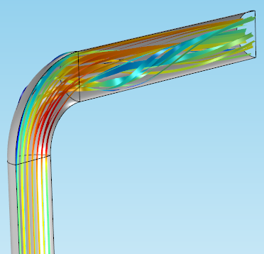
In the solved model, there is an existing 3D plot group called Pressure (spf2) that already contains a streamline plot. Let’s take a look:
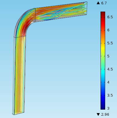
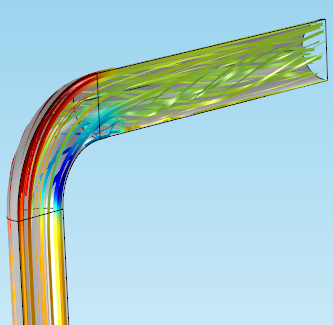
Only half of the symmetric pipe geometry is modeled, with the inlet at the bottom and the outlet at the top right in this view. The streamlines in this plot group show the instantaneous fluid velocity as water flows toward, through, and away from the bend. We can see a fully developed turbulent flow profile at first; then, a separation zone and turbulent vortices appear after the bend. The color expression in the streamline plot indicates fluid velocity (in m/s).
There are several different ways to arrange streamline plots. In the settings window, the Streamline Positioning tab contains different options for the position. We’ll touch on just a few of them.
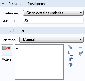
In the figure previously shown, the positioning is set to On selected boundaries, meaning that a single boundary has been selected for the curves to start at — in this case, the inlet of the pipe — and the user specifies how many streamlines to plot. Currently, there are twenty individual curves released that begin at this boundary, as specified in the Number field:
Streamline Styles
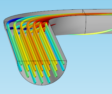
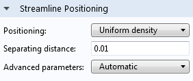
Some of the other positioning tools have slightly different effects. I’ll now set the positioning to Uniform density. With this option, the user controls the distance between each curve rather than specifying the number of lines.
This is also where, if you’re not careful, you might end up with a very dense array of streamlines, which can take some time to compute the postprocessing:
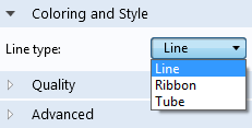
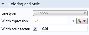
The presentation of the streamline density can be adjusted using the tube settings under the Coloring and Style tab. We can either shrink the tube radius (currently set to 0.001 m) or choose a different line style from the Line type drop-down list.
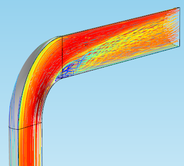
For a case like the dense uniformity shown in the previous figure, the line style will show the plot more clearly than the tubes with the radius shown above:
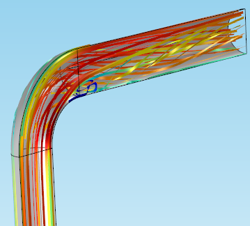
The ribbon style shows the streamlines as flat ribbons. Like the tube style, these are controlled by a user-defined width and scale factor. Both styles share the risk of the same density issue if they are packed together too tightly. For the figure below, I increased the separating distance from 0.01 to 0.02, thereby decreasing the number of ribbon streamlines plotted:
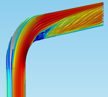
One nice trick you can do with the ribbons, especially for RANS CFD applications, is to set the ribbon width to a variable. I have set the width expression (scaled down) to k2, representing the turbulent kinetic energy.
This can be used to help identify vortices in the flow. Below, we can see that the ribbons are much thinner before the bend. They thicken near the bottom of the pipe after the elbow, where the turbulent kinetic energy has increased:
Coloring Streamlines to Show Physical Results
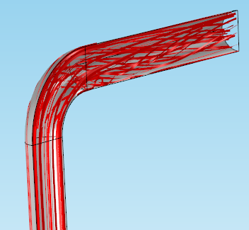
We’ve now seen a few different ways to shape the streamlines, but what are they really representing? Often, one of the best uses for streamlines is to depict the flow velocity as fluid moves through a domain — in this case, the pipe bend. Each of the earlier examples shows a plot that, by default, contains a color expression. Disabling this color expression from the streamline plot will show a very different look. The result is still useful as it shows the turbulent flow in the pipe, but it doesn’t provide the same information (and this is why coloring is so significant):
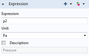
Let’s take a look at the Color Expression settings. Like most plots, the color expression will be based on a variable of your choice. The variable you choose depends on your application. For this model, it’s important to know the velocity and fluid pressure of the water. I’ll set the expression to show pressure:
Below, you can see how the coloring looks different than it did earlier when it was set to show velocity. This image also shows the extent of the pressure drop brought on by the fluid being forced through a 90-degree bend:
There you have it. We have provided you with a brief example of how streamline plots can be particularly helpful in depicting fluid flow — which could mean air, water, or a chemical mixture — through any domain. I hope you’ll have the opportunity to apply this technique in your future postprocessing efforts.
Further Reading
- Download the Flow in a Pipe Elbow model
- Read the previous blog entry in this postprocessing series

Comments (3)
andreas pelapelapon
January 2, 2015I am really a beginner
I wish someone may send me the application library of fluid flow in a sea cooling water system
Thank you, and happy new year
Lexi Carver
January 6, 2015Hi Andreas,
I have a few different suggestions for what you might be looking for. If you’re modeling a conjugate heat transfer application, I suggest browsing through the models here: http://www.comsol.com/models/heat-transfer-module. These are all shipped with the Heat Transfer Module, an add-on product to COMSOL Multiphysics.
If you’re looking for something a little different, more models using fluid flow can be found here: http://www.comsol.com/models/cfd-module and here: http://www.comsol.com/models/pipe-flow-module, for the CFD and the Pipe Flow Module, respectively.
The models are fully documented in the PDFs, so you can take a look at the model setup before downloading them. There’s plenty of models available in the Model Gallery, so I hope you’ll find one similar to your application.
Best regards,
Lexi
Xiaoguang Yin
June 11, 2019I have to say, this post is not that helpful. For example, for “Uniform density”: “the user controls the distance between each curve rather than specifying the number of lines”, what does this mean, ” distance beween each curve ” , spatial distance or some distance definition based on the velocity field?