Centre d'apprentissage

Meshing MHD Models For Efficient Simulation

---

The previous parts of this course focused on setting up the physics interfaces for a magnetohydrodynamics (MHD) model in the COMSOL Multiphysics^® software. After setting up the interfaces, it's important to make sure that the simulation solves accurately and efficiently, minimizing memory use and computation time. There are two main parts to achieving this: building an efficient and accurate mesh and then configuring the solver to work efficiently.

This article will cover techniques that can be used to mesh MHD models for efficient simulation. The next part of the course will discuss solver techniques.

Meshing Magnetohydrodynamics Models

Meshing MHD flow models draws on many of the standard meshing techniques for CFD problems, which you can find more information on in these articles: How to Set Up a Mesh in COMSOL Multiphysics® for CFD Analyses and Your Guide to Meshing Techniques for Efficient CFD Modeling.

The key goals in meshing an MHD flow model are:

• For laminar flow in ducts, the solution changes minimally along the length of the pipe, while the gradient of the flow profile is steeper in the plane of the cross section of the flow. The mesh should resolve the flow at both these length scales efficiently.
• The boundary layers, and any jets or areas of reversed flow, should be well resolved in the flow profile.
• The mesh should be refined enough that the solution is independent of small changes in the mesh. The discretization of the problem should not affect the solution.

The first goal can be achieved by using a swept mesh, which generates anisotropic mesh elements, allowing them to be longer parallel to the direction of flow. For a course dedicated to building swept meshes, see Using Swept Meshes for Model Geometries.

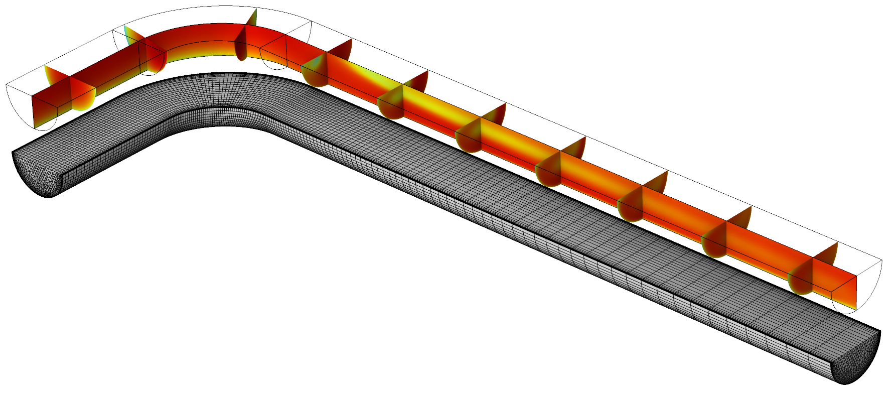
An example of a simple hydrodynamics model, the Flow Through a Pipe Elbow tutorial, showing a system where a swept mesh is beneficial. The cross section needs to be meshed with a finer mesh size, especially near the walls to resolve the gradient of the solution. The mesh discretization along the flow gradually increases in size as the gradient of the velocity in this direction becomes smaller. (Each cross section exhibits approximately the same velocity profile.)

There are two methods for handling the resolution of the boundary layers, jets, and reversed flow. 

Outside of cases where swept meshes can be used, the easiest method of resolving boundary layers is to use the standard CFD method of adding a Boundary Layer mesh to all of the wall boundaries. The thickness of the boundary layer elements can be set to resolve the Hartmann layers, which are a type of boundary layer that develop in flow next to walls where viscous and Lorentz forces are in balance.

A tutorial series on generating boundary layer meshes is available here: Boundary Layer Meshing Tutorial Series

The second resolution method is specific to duct or pipe flow models that use swept meshes. In these cases, the options that COMSOL Multiphysics^® provides for building user-defined meshes can be used to develop a custom mesh for the cross section, which provides the required resolution of the boundary layers, jets, and reversed flow. 

Resolving the flow profile in the cross section of a duct requires resolving each of the key features of the flow, which involves both rapid changes in the magnitude and the gradient of the flow in the boundary layers as well as a core area where the flow is relatively constant.

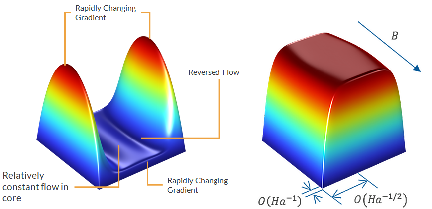
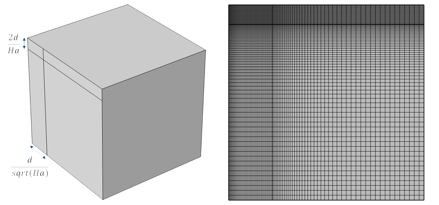
The image on the left displays the flow profile for square duct flow when the side walls are insulating and the Hartmann walls are conducting for a high Hartmann number. The key features that need to be resolved are shown. The image on the right shows the thickness of the Hartmann layers in a duct with insulating walls parallel and perpendicular to the magnetic field, demonstrating the anisotropic behavior.

An efficient mesh for this problem would use large mesh elements in the core, where the flow is mostly constant, and then target the areas with rapid changes in the gradient with smaller mesh elements. In addition, because the flow profile and gradients are anisotropic in the directions parallel and perpendicular to the magnetic field, an efficient mesh would also allow for anisotropic mesh elements whose size can be independently controlled in each direction.

These requirements are best satisfied by the Mapped mesh. The mapped mesh places a structured mapping of a rectangular grid of mesh elements across a 2D surface, and by premeshing the perimeter edges using Edge mesh nodes, the size of the mesh elements can be controlled.

A Free Triangular mesh applied to the boundary (left) and a Mapped mesh using anisotropic elements (right).

The simplest method of using a mapped mesh to resolve the cross-section flow is to define it across the cross section of the duct, using Distribution nodes to control the size of the mesh elements. With the Predefined setting in the Distribution node, the total number of elements along the edge, the ratio of the smallest to largest elements , and whether the element sizes follow the pattern of a linear or exponential sequence are set. This creates a grid of elements whose size changes smoothly, with thin elements placed in the Hartmann layers of the fluid to resolve the flow.

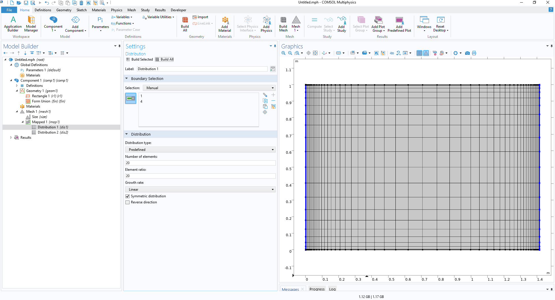The Settings window for a Distribution node where the element size is set. Using a Distribution node to set the horizontal mesh element size to follow a symmetric exponential sequence and the vertical mesh element size to follow a symmetric linear sequence. In both directions, a total of 50 elements is used, with an element ratio of 20.

The linear and exponential sequence equations can be used to identify the relationship between the sizes of each element from and . The image below identifies the parameters for an asymmetric and a symmetric distribution.

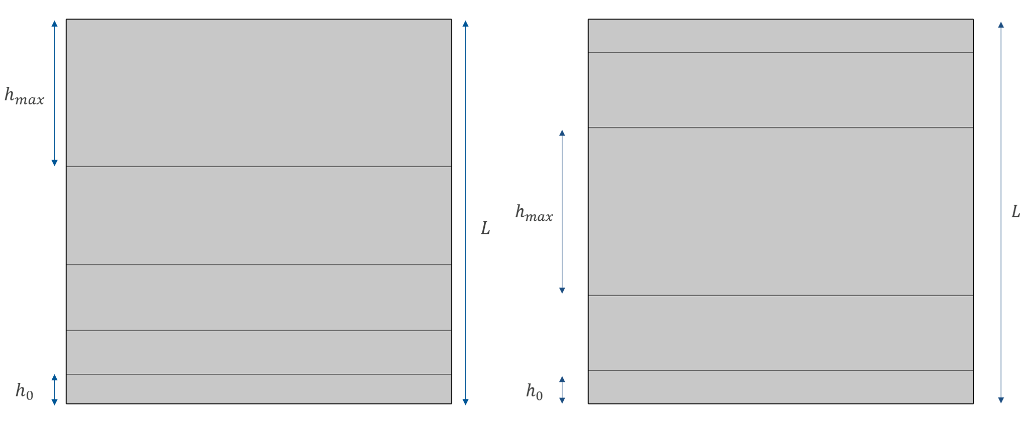
Definition of the different lengths for an asymmetric (left) and symmetric (right) distribution. The total length is noted as .

For the above image, the element sizes are related as:

Expression	Linear	Exponential

In order to resolve the Hartmann layers, it is desirable to set the thickness of the first element to be a fraction of the thickness of the Hartmann layer. Using a distribution, this requires identifying and , which produce the desired . This is possible, but it is often easier to use a second method where the edges are meshed prior to using the Mapped mesh, using a Size node to control the thickness of the first layer.

To follow this method, create an Edge mesh and apply it to one of the edges that is being meshed. Two Size attributes are then added to the Edge mesh. The first is applied to the boundaries that are being meshed. Here, the general maximum and minimum element sizes for the entire edge are set, along with the maximum element growth rate. 

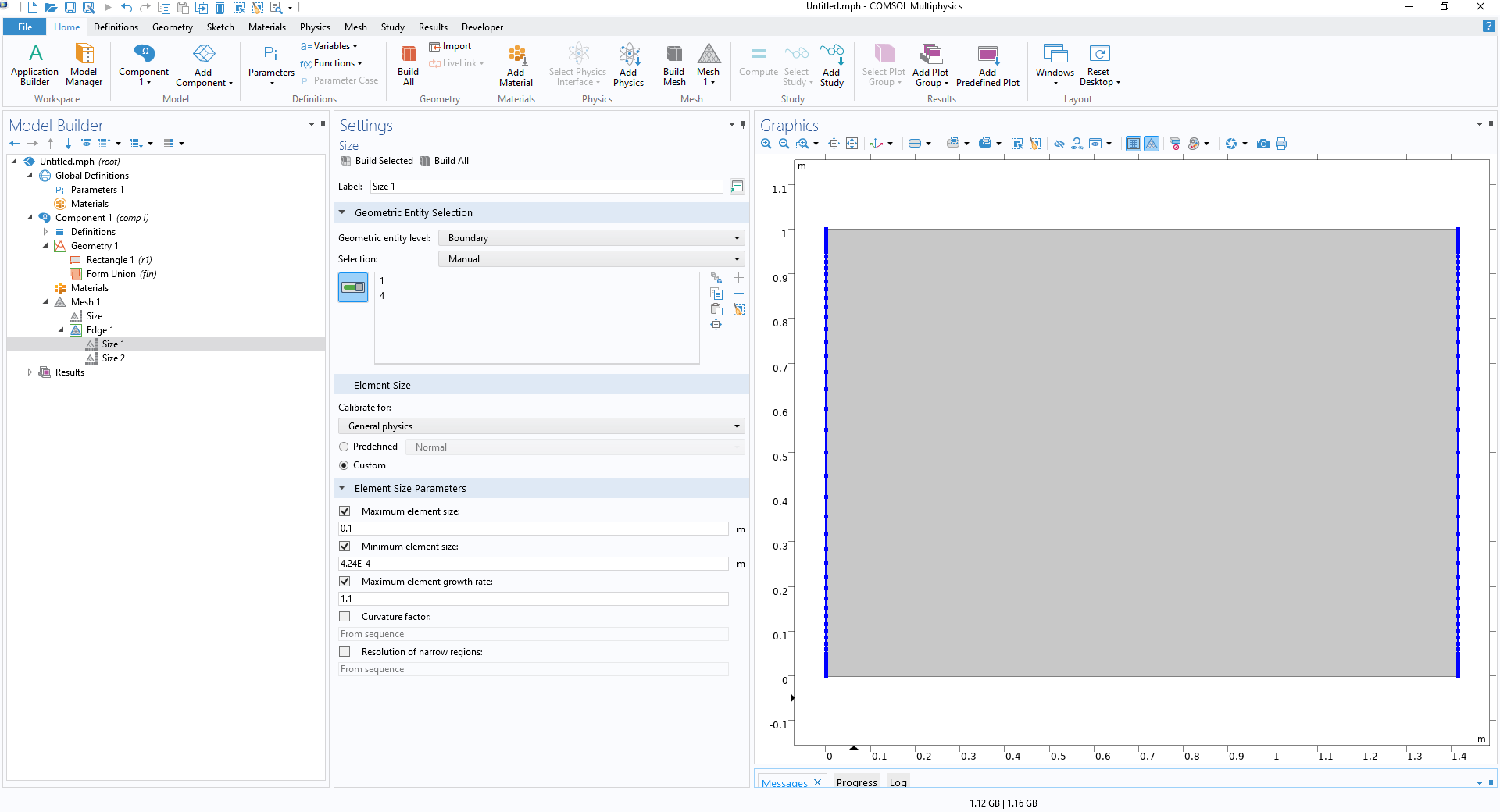The Size Settings window is open to set the constraints of element size and growth rate. The first Size node to constrain the maximum element size and the growth rate on the edges being meshed.

The second Size attribute is used to set the size of the first element by applying it to a vertex or edge that passes through the vertex that is neighboring this first element. The maximum and minimum element sizes should both be set to the desired first element thickness.

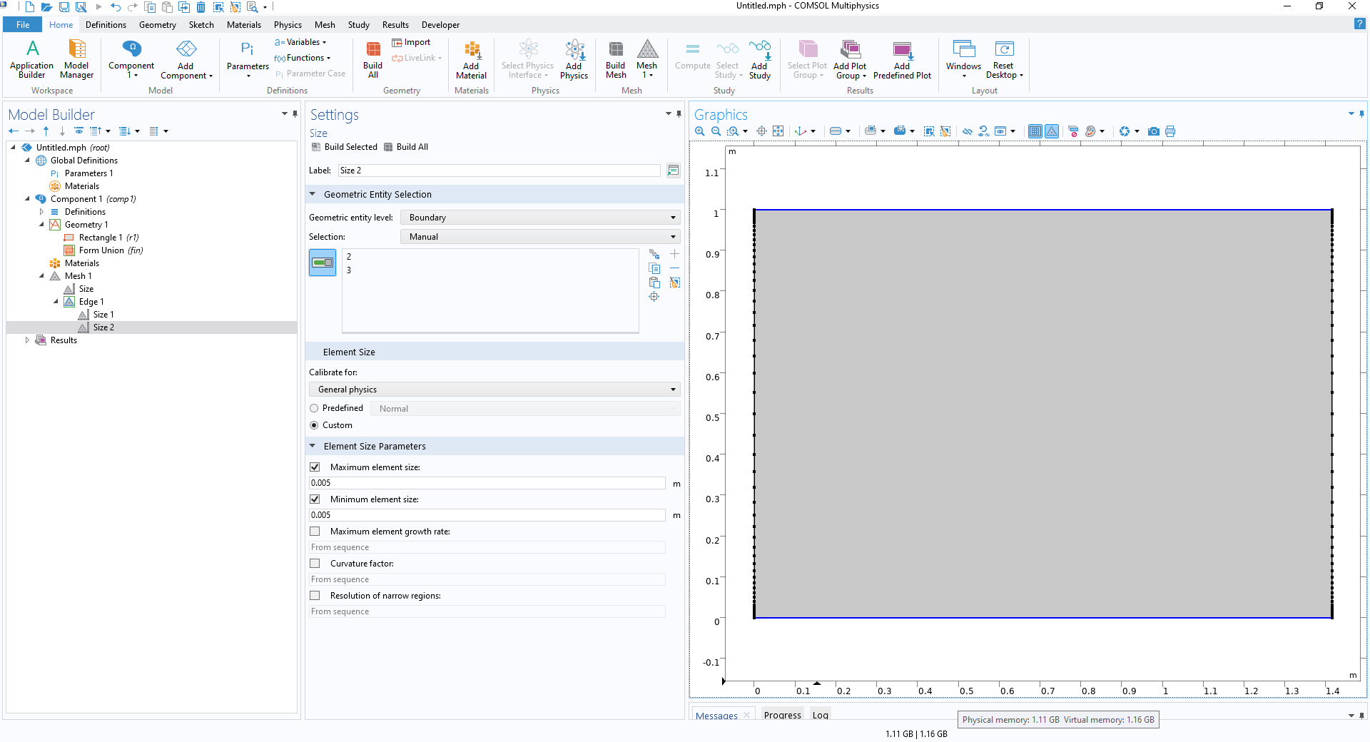A Size Settings window is used to add further constraints. The second size constraint used to fix the thickness of the first element next to the wall to 0.005 m by constraining the adjacent edges.

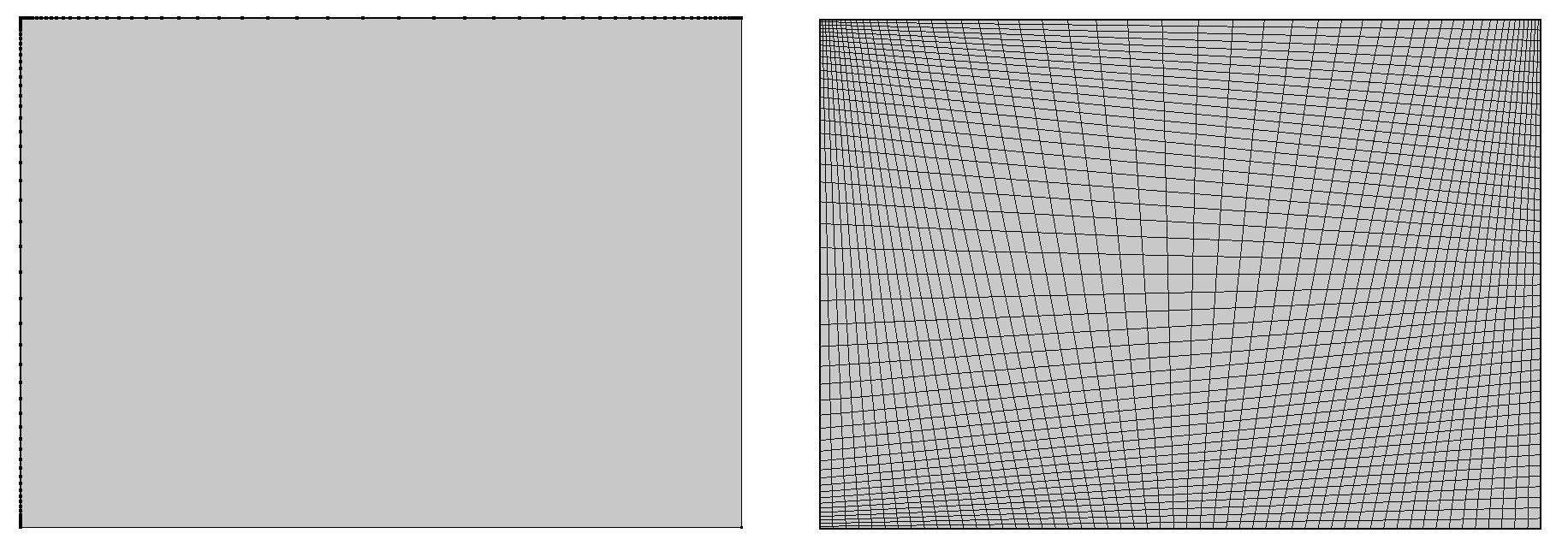
This process can be repeated to mesh the remaining edges to form a perimeter mesh, and then the Mapped mesh can be applied to create the boundary mesh for the cross section.

The completed perimeter mesh (left) and the result of applying the Mapped mesh (right).

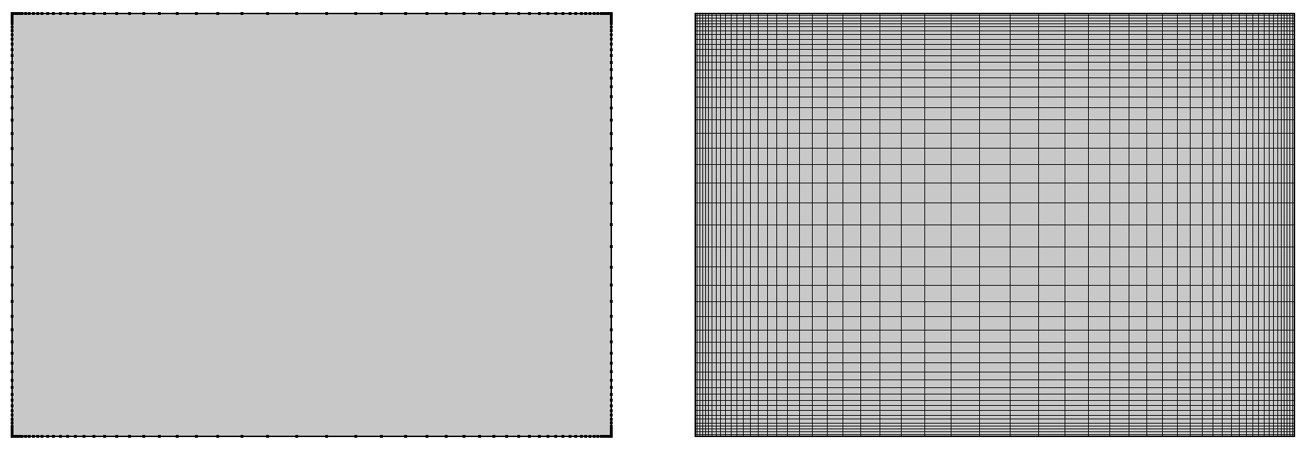
It is important to ensure that all of the edges are meshed prior to applying the Mapped mesh; otherwise, the mesh generator will default to applying a uniform distribution of elements to the unmeshed edges. This leads to heavily distorted grids of elements. 

Left: meshing only two edges of the rectangle, one horizontal edge and one vertical edge, prior to applying the mapped mesh. Right: the generated mapped mesh, showing uniform element distribution on the two edges, which were not premeshed, creating a very poor mesh.

The benefit of the second method is that it can be combined with partitioning the cross section into different areas with different size constraints applied to different areas. When the edge mesh is applied, the growth between elements will always be smooth, as is required for a good MHD cross-section mesh. The Distribution method will not create smooth mesh transitions, creating exactly the mesh element size distribution specified in it and thus creating discontinuities in the element growth, which can affect the solution. 

The partitioning of the Hartmann layers out of the core of the cross section by using the scaling relationships for them, for a square duct where the two possible symmetry cuts have been made (left). The mesh created by specifying finer mesh elements in the partitions (right).

When there are jets or areas of reversed flow in the model, it is also possible to partition these regions for denser meshing. Below, a suitable vertical partitioning and meshing of the cross section is identified to resolve a duct flow with jets.

Three images showing a plot of the normalized flow profile, where the partitions might be created, and the mesh. A solution for duct flow with jets is plotted and divided into four parts where the mesh needs different levels of resolution. Those parts correspond with the two sides of the jet, the peak of the jet, and the core of the fluid (left). The geometry has matching partitions added to the cross section (center). The horizontal mesh size in each partition is set to the appropriate level of resolution, with the smallest elements directly next to the boundary wall and at the peak of the jet and the largest elements in the core of the fluid (right).

The position of these partitions can also be functions of the Hartmann number. This function may already be known. For instance, in the case of square duct flow with conducting Hartmann walls, the peak occurs at approximately a distance from the side wall, and this distance can be used to define the partitioning. 

Cases where this relationship is not known can require some trial and error in identifying where to place the partition and how large it should be — a coarse mesh may predict one position and width of the jet, but when the mesh is refined to resolve it better, the new solution may indicate some error in these predictions. The partitions should then be updated, and the model rerun. Only once the jets retain their position relative to the partitions should the partitioning of the mesh be considered suitable. This also provides the first step of evaluating the mesh for accuracy.

For nonrectangular ducts, it can also be necessary to partition the cross-section face in order to be able to apply the Mapped mesh, as it can only be applied to boundaries that are topologically equivalent to rectangles. This prevents it from being applied directly to circular or elliptical cross sections, for example. It is possible to use the Mapped mesh on the majority of the cross section by partitioning out the central core of the fluid, applying the Mapped mesh to the outer rings this creates, and then applying a Free Quadrilateral mesh to the central core. 

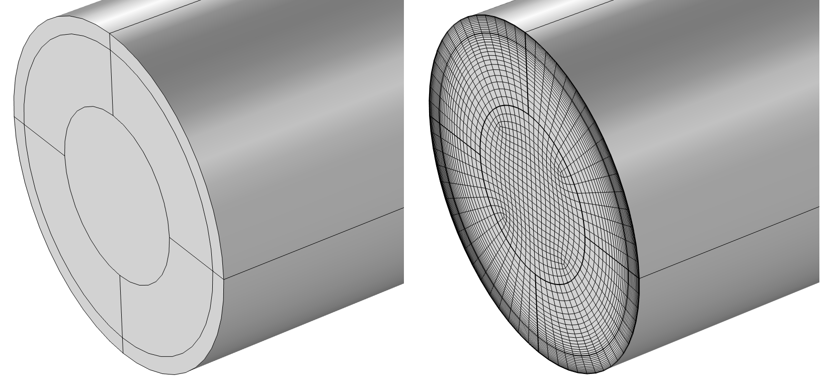
Sections of a circular pipe have been partitioned out for the boundary layers, core, and intermediate areas (left). A Mapped mesh is applied in the two outer regions and a Free Quadrilateral mesh is applied in the core (right). The size of the core region has been chosen so that the elements are approximately square within the entire region.

Evaluating the Mesh

While any mesh will generate a solution to the problem, it is necessary to ensure that the mesh is sufficiently resolving the solution to generate an accurate solution, and that the returned solution does not have any dependency on the mesh so that features of the solution will not change if the mesh is changed slightly. 

The accuracy of the mesh can be improved by reducing the size of the elements used to construct it. If the value of an output is tracked on a series of successively finer meshes, it will be seen to tend to a limit — the predicted true value. 

The process of calculating this limit is known as performing a mesh refinement study (See our article Performing a Mesh Refinement Study to learn about methods for automatically converging the mesh and manually refining the mesh.) When working with Mapped and Swept meshes, which are structured, the manual techniques of parameterizing and changing the maximum and minimum element sizes in a Size node are preferred, as this will preserve the structure of the mesh, whereas the adaptive mesh refinement method would not.

It should be noted that when attempting to benchmark models to an analytic solution, the limiting value for the solution found through mesh refinement may retain a small error compared to the analytic value. The solver settings also contribute to the accuracy of the solution and will provide a lower limit to the error found when comparing the simulated values to the analytic values that cannot be reduced through mesh refinement. Instead, the solver settings can be adjusted to lower this error.

This can be seen in the preview image below, where mesh refinement is performed on an MHD model using two different solvers: the default solver and one that has been adjusted to improve its accuracy. The same set of meshes is used for each of the mesh convergence studies, and identical convergence to a limit is seen — the solution is just translated by an error. It is seen that using the default solver, the predicted maximum normalized fluid velocity deviates from the analytic expression by . This error is reduced by using the adjusted and improved solver, which converges to a value much closer to the analytic solution. 

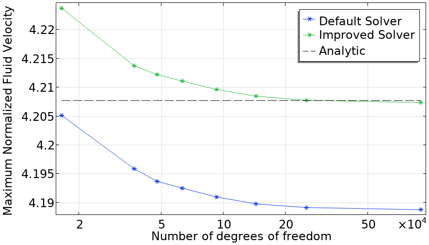
Comparing the mesh refinement outcomes for a model running with the default solver and a solver with an improved configuration.

In the next part of the course, the adjustments to the solvers used to generate the image above will be covered.