Modeling Acoustic Ray Tracing: Release from Pressure Field
In the previous parts, we examined two methods for defining a point ray source with a speaker's directivity to model its behavior in a room using ray tracing. In this part, we continue with the same room setup and begin exploring the first of two methods using a surface ray source to characterize a speaker's output in ray acoustics analysis. Both methods require acoustic intensity data, including the direction and magnitude of the local intensity, on a surface where rays are released. Similar to the point ray source options, the data can come from either measurements or simulations. For the latter, a wave-based FEM analysis must first be conducted to solve the acoustic field within the source region. This allows for the inclusion of nearby geometry details along with the speaker in the source model, so the surface source also accounts for scattering effects from the closest corners or edges. In this part, we use the terms "release surface" and "radiating surface" interchangeably to refer to the "source surface."
The article "Using Acoustic Ray Tracing to Model Speaker-Room Performance" provides context for this article.
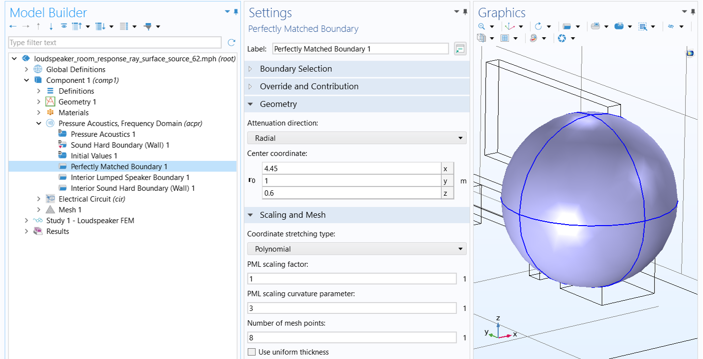
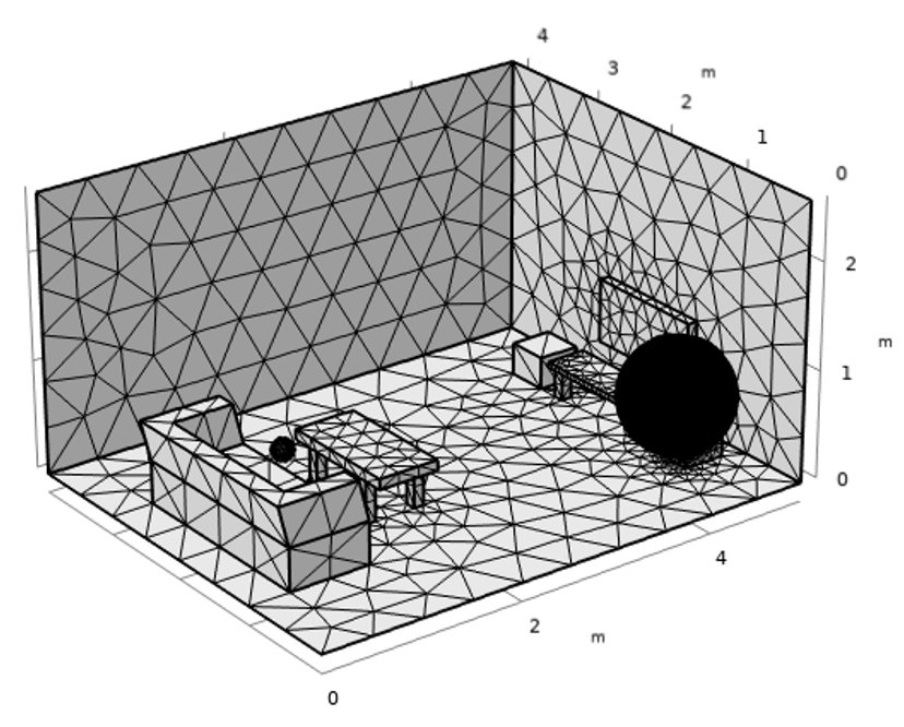
From versions 6.2 and up, you can use the direct FEM to ray coupling feature, Release from Pressure Field. The FEM source model and the ray acoustics model should be set up in the same component within the same model. We are using the same geometry from the FEM room acoustics analysis conducted in Part 1, with the addition of a sphere to create a source region, highlighted in blue in the image below, where the source model will be solved. The sphere, centered exactly where the point ray source is defined in Part 3, has a radius of 0.525 meters. This size is chosen to ensure that the full-wave source model remains manageable while still encompassing the boxed speaker and some nearby table edges.
 A room and furniture represented by gray geometry with a blue sphere containing the source speaker.
The geometry used for the analysis conducted in this part. The source model is solved within the sphere (highlighted in blue), which encloses the speaker box and some nearby surfaces.
A room and furniture represented by gray geometry with a blue sphere containing the source speaker.
The geometry used for the analysis conducted in this part. The source model is solved within the sphere (highlighted in blue), which encloses the speaker box and some nearby surfaces.
It is important to note that when rays are emitted from a boundary, they are all launched simultaneously. As a result, it is assumed that the sound from the source arrives at and departs from every point on the release boundary at the same time. For this assumption to hold, the release boundary must be positioned carefully and cannot be chosen arbitrarily. Here, the center of the release surface is aligned with the location of the point ray source defined in Part 3.
Let's first set up the source model.
The Source Model
The image below offers a close-up view of the geometry used for the source model, enabling the calculation of the near-field solution that includes diffraction effects from nearby table surfaces and corner edges. The entire surface of the sphere, excluding the portion that intersects with the tables, acts as the radiating surface and serves as the release surface in the ray acoustics model. All boundaries defining the release surface are grouped into a selection called "Release Boundaries."
 A close-up of the transparent blue sphere surrounding a gray source speaker in a gray room.
A close-up view of the geometry used for the source model.
A close-up of the transparent blue sphere surrounding a gray source speaker in a gray room.
A close-up view of the geometry used for the source model.
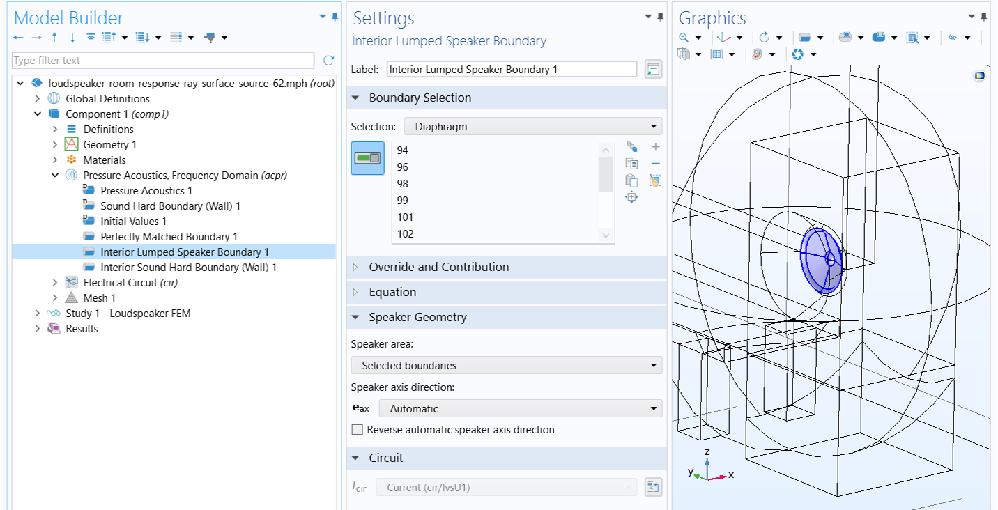
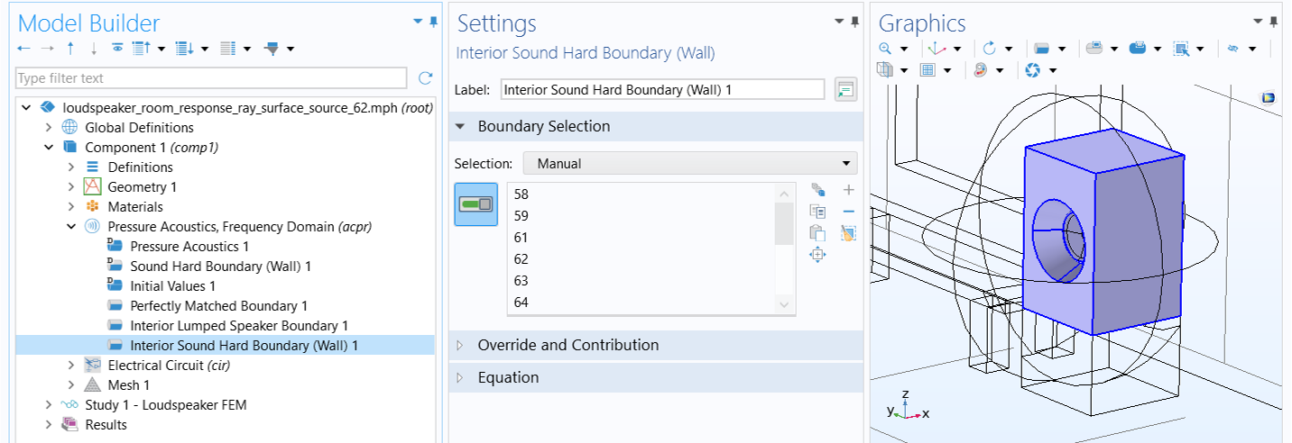
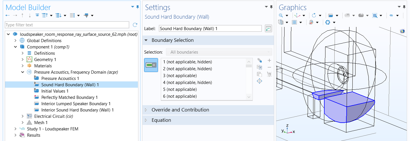
As in Part 3, the source model uses the Pressure Acoustics, Frequency Domain interface, with the driver represented by a lumped circuit. The circuit is coupled to the FEM acoustic domains—both inside and outside the speaker box—at the diaphragm's location through the Interior Lumped Speaker Boundary feature. The radiating surface is modeled with the Perfectly Matched Boundary feature, while all surfaces of the box enclosure, except for the diaphragm, are represented as sound-hard walls using the Interior Sound Hard Boundary condition. The nearby table surfaces included in the model are also simulated as sound-hard walls, which is the default setup due to their role as exterior boundaries of the acoustic domains. The relevant boundary settings are illustrated in the images below. Note that in the Perfectly Matched Boundary settings, the Center coordinate in the Geometry section must be specified correctly for optimal performance of the condition.
Also, ensure that in the External Device section of the External I vs. U 1 node within the Electrical Circuit interface, Electric potential is set to Voltage from lumped speaker boundary (acpr/ilsb1) to couple the pressure acoustics model back to the lumped speaker model. This setting accounts for the effect of pressure load on the speaker's diaphragm.
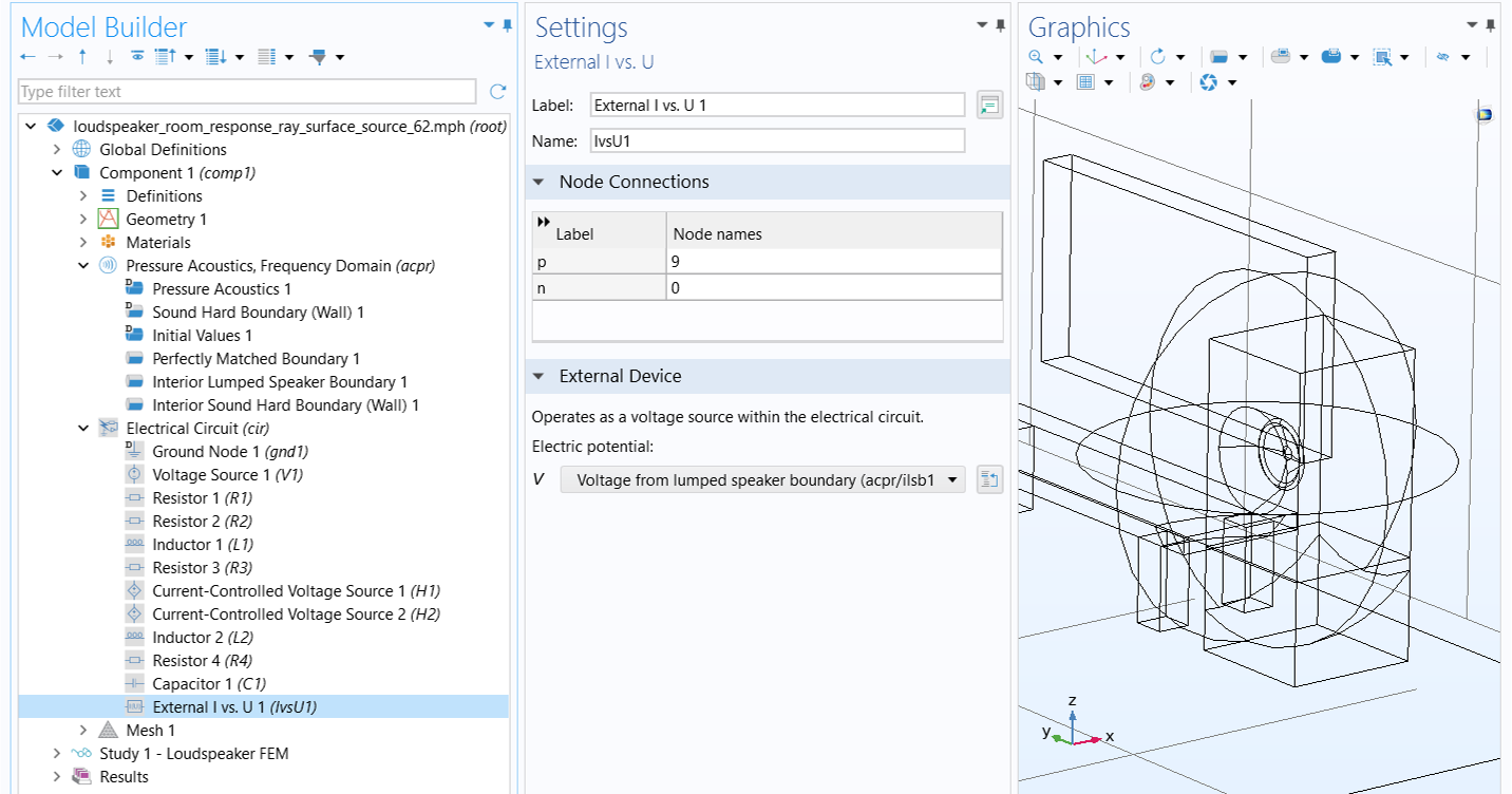 The External I vs. U settings configure the external device as a voltage from the lumped speaker boundary.
The setting in the External I vs. U node incorporates the effect of pressure load on the speaker's diaphragm in the lumped speaker model.
The External I vs. U settings configure the external device as a voltage from the lumped speaker boundary.
The setting in the External I vs. U node incorporates the effect of pressure load on the speaker's diaphragm in the lumped speaker model.
The source region is meshed with the Free Tetrahedral element type to resolve wavelengths up to 4000 Hz, which is necessary for solving the wave-based FEM source model. Surfaces outside the sphere are meshed with the Free Triangular element type for the subsequent ray acoustics analysis, using predefined Normal size settings. However, a mesh size of Rr/3 is applied to the receiver surfaces to resolve the spherical shape, where Rr is the radius of the receiver.
 A very fine tetrahedral mesh is applied on the spherical source and a course triangular mesh is applied on the other surfaces.
The source region inside the sphere is meshed for FEM analysis of the source model, while the external surfaces are meshed for ray tracing study.
A very fine tetrahedral mesh is applied on the spherical source and a course triangular mesh is applied on the other surfaces.
The source region inside the sphere is meshed for FEM analysis of the source model, while the external surfaces are meshed for ray tracing study.
Like in Part 3, the source model is solved in the frequency domain from 125 Hz to 4000 Hz, using 1/3 octave intervals. The results shown below depict the acoustic intensity vectors and magnitude on the radiating surface for the selected frequencies.
 Four plots of the source sphere at different frequencies use colored surface plots and gray arrows.
Intensity direction and magnitude on the release surface.
Four plots of the source sphere at different frequencies use colored surface plots and gray arrows.
Intensity direction and magnitude on the release surface.
The blue solid line in the image below depicts the total radiated power from the radiating surface as a function of frequency, calculated by integrating the outgoing acoustic intensity over the release boundaries. This is in good agreement with the radiated power calculated by the Interior Lumped Speaker Boundary node (represented by green circles), stored in the variable acpr.ilsb1.P_front.
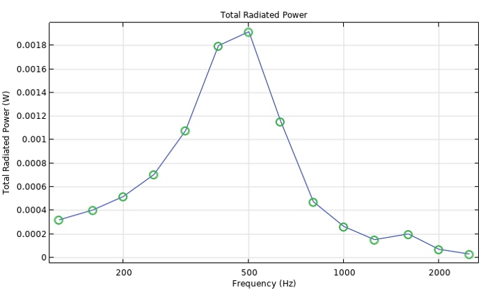 A graph of the total radiated power in watts versus frequencies from 125 to over 2000 Hz.
The total radiated power from the radiating surface as a function of frequency.
A graph of the total radiated power in watts versus frequencies from 125 to over 2000 Hz.
The total radiated power from the radiating surface as a function of frequency.
The Ray Acoustics Model
To use the Release from Pressure Field feature, add a Ray Acoustics physics interface to the same component within the same model as the FEM source model. A brief overview of the ray model settings identical to those in Part 3 is provided below. For more detailed information, please refer to the "Ray Acoustics Model Using Release from Exterior Field Calculation" section in Part 3.
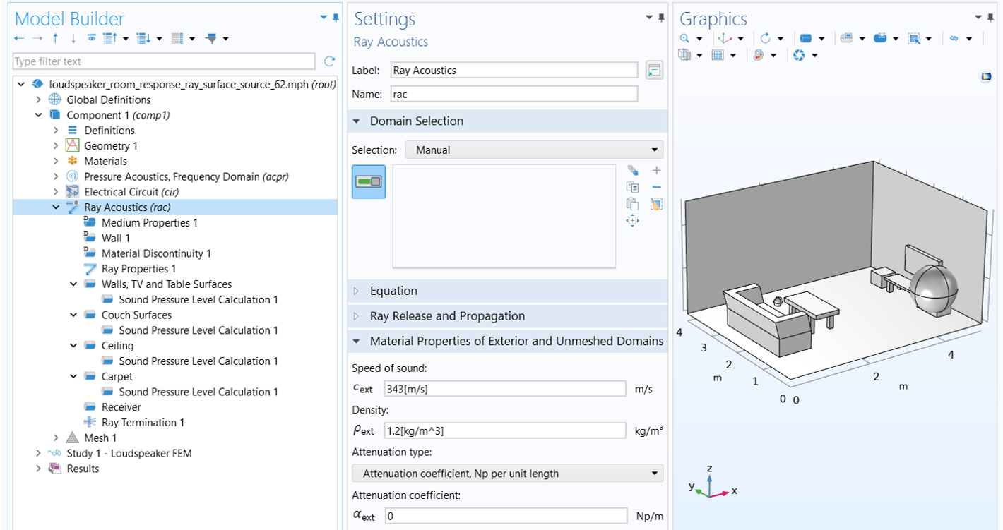
1) The Ray Acoustics interface does not include any domain in its selection. This allows us to only mesh the surfaces where a boundary condition is applied. We use the default acoustic properties specified for all unselected domains in the Material Properties of Exterior and Unmeshed Domains section. Compute Intensity and power is selected for Intensity computation in the Intensity Computation section, and Count Reflections is selected in the Additional Variables section. These settings ensure the access to the Release from Pressure Field and Receiver features within the physics interface, as well as the Impulse Response analysis during postprocessing.
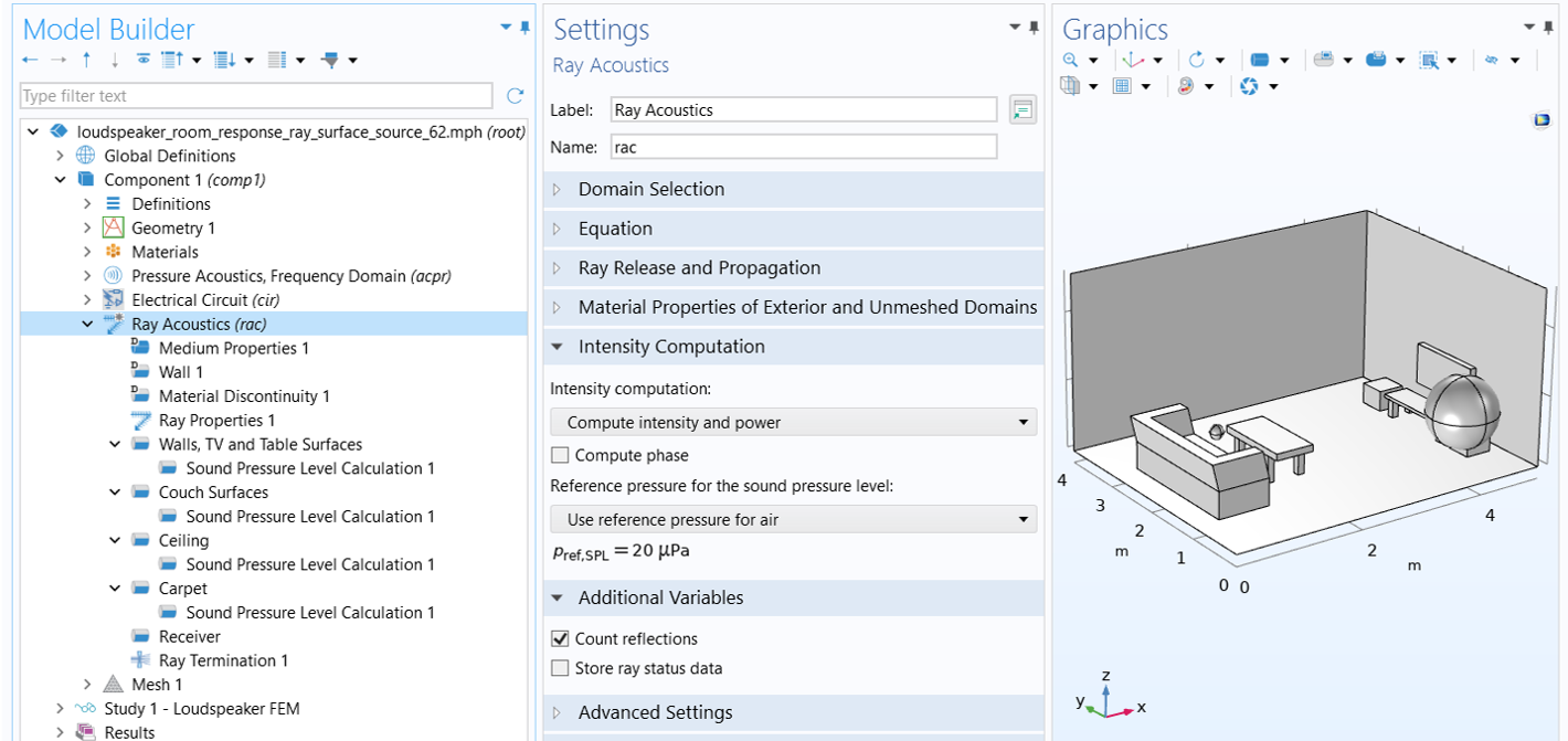
2) In the Ray Properties 1 node, set Ray frequency to f0.
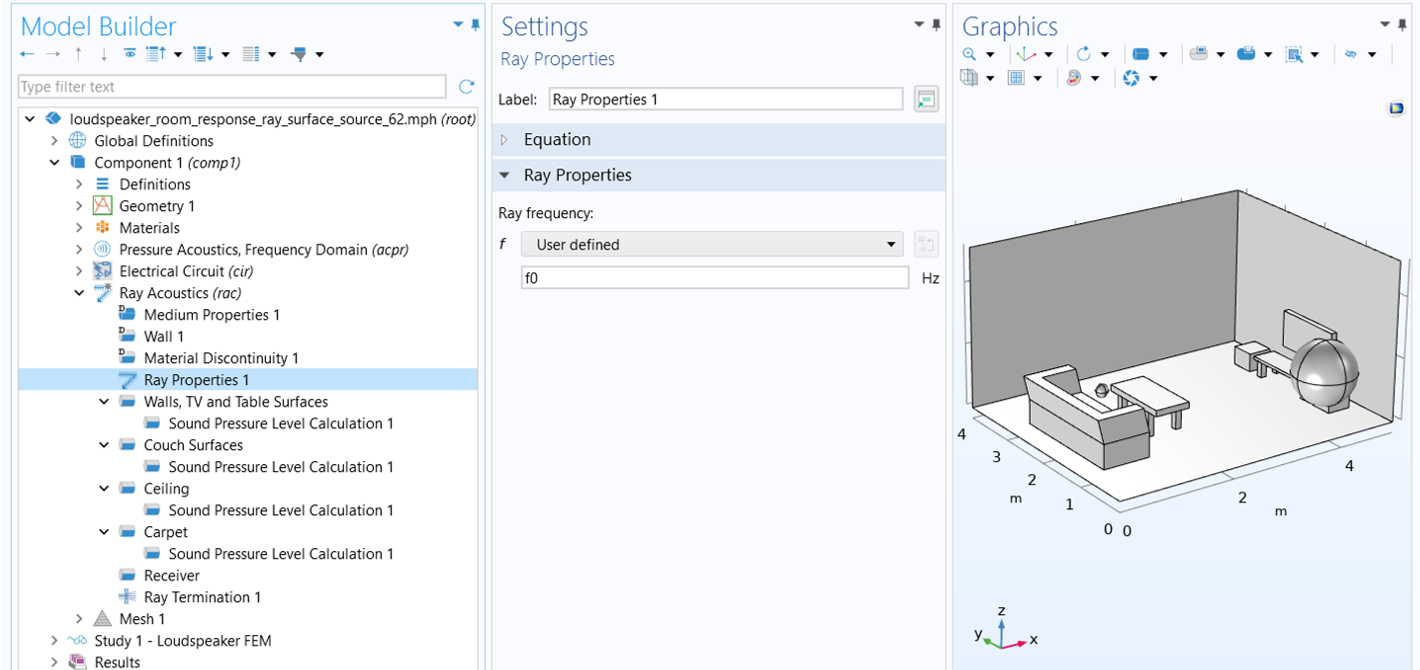 The user defined ray frequency in the ray properties settings window.
The ray frequency setup.
The user defined ray frequency in the ray properties settings window.
The ray frequency setup.
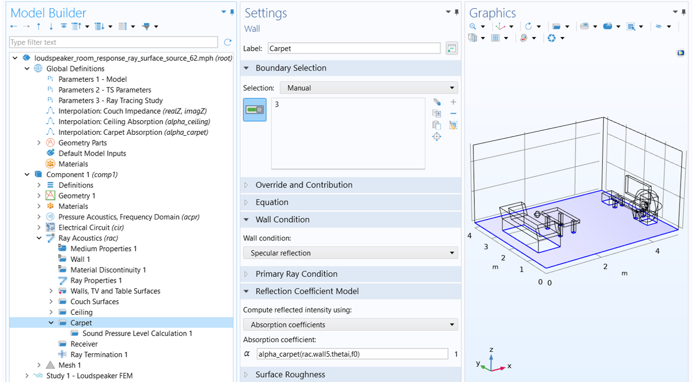
3) All surfaces, except for the couch, ceiling, carpet, and receiver surfaces, are defined using the Specular Reflection wall condition with a constant absorption coefficient of 0.1. A Sound Pressure Level Calculation subnode is used to compute the sound pressure level on those surfaces.
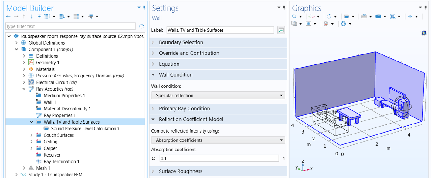 The hard surfaces of the room are highlighted in blue and the absorption coefficient is set in the settings window.
Walls and surfaces of the TV, speaker box and tables are modeled as specularly reflecting walls with a constant absorption coefficient.
The hard surfaces of the room are highlighted in blue and the absorption coefficient is set in the settings window.
Walls and surfaces of the TV, speaker box and tables are modeled as specularly reflecting walls with a constant absorption coefficient.
4) The couch surfaces are modeled as absorbers using the Specular Reflection wall condition with frequency-dependent impedance. The impedance data are imported via two interpolation functions: realZ for the real part and imagZ for the imaginary part. Since these data represent the acoustic impedance relative to air, it must be multiplied by the impedance of air to obtain the characteristic impedance. A Sound Pressure Level Calculation sub-feature is applied to the couch surfaces to compute the sound pressure level.
 The couch is highlighted in blue and set as an absorber in the settings window.
Couch surfaces are modeled as absorbers with frequency-dependent impedance.
The couch is highlighted in blue and set as an absorber in the settings window.
Couch surfaces are modeled as absorbers with frequency-dependent impedance.
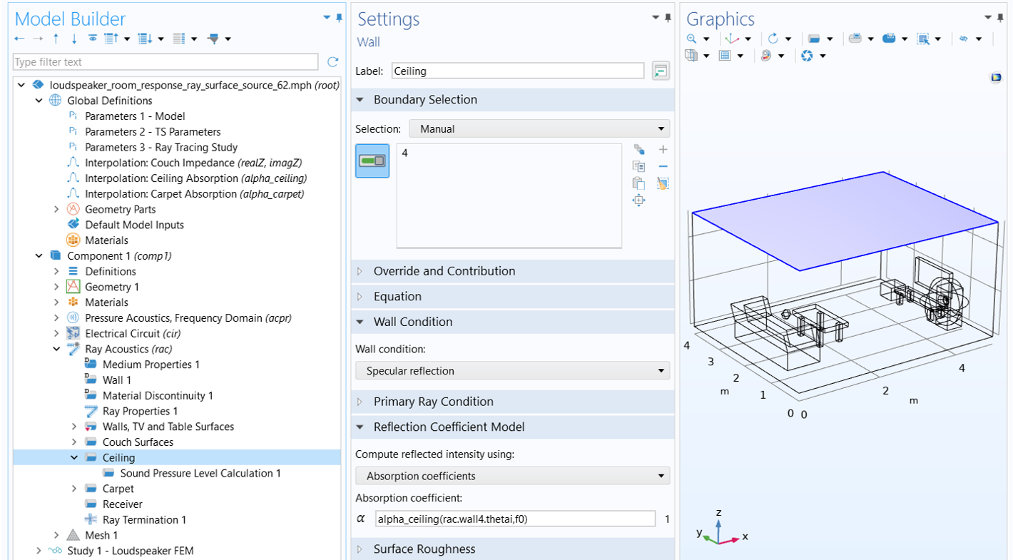
5) The absorption of ceiling and carpet is modeled using frequency- and angle-dependent absorption coefficients. These coefficients are computed and exported from the Acoustic Treatment Boundary Calculator app, and imported via two interpolation functions: alpha_ceiling for the ceiling and alpha_carpet for the carpet. Sound pressure levels are also calculated on these two surfaces.
6) The physics-based Receiver feature is used and the condition is applied to the surfaces of the receiver sphere located above the couch. This allows for faster impulse response calculation in the results analysis.
 The sphere is selected in blue within the wireframe room geometry and set as an omnidirectional receiver.
The physics-based * Receiver * setup.
The sphere is selected in blue within the wireframe room geometry and set as an omnidirectional receiver.
The physics-based * Receiver * setup.
7) The Ray Termination feature is used to remove rays from the model when they exit the geometry.
 The ray propagation is set to stop at the bounding box of the geometry.
Ray termination setup.
The ray propagation is set to stop at the bounding box of the geometry.
Ray termination setup.
The Surface Ray Source Setup Using Release From Pressure Field
Let's now look at how to use the Release from Pressure Field feature to define a surface ray source that represents the output from the speaker. After adding the node to the Ray Acoustics interface, select Release Boundaries from the Boundary Selection list to apply the feature to the entire release surface. Then, in the Solution Field section, choose Pressure Acoustics, Frequency Domain (acpr) for Physics interface. Finally, in the Release from Pressure Field section, enter the parameter Nrays to specify the number of rays per release. As in Part 3, Nrays is set to 20,000.
 A blue sphere surrounds the wireframe of the speaker within the wireframe room geometry.
The Release from Pressure Field feature enables direct FEM-ray coupling to define a realistic speaker source in ray tracing analysis.
A blue sphere surrounds the wireframe of the speaker within the wireframe room geometry.
The Release from Pressure Field feature enables direct FEM-ray coupling to define a realistic speaker source in ray tracing analysis.
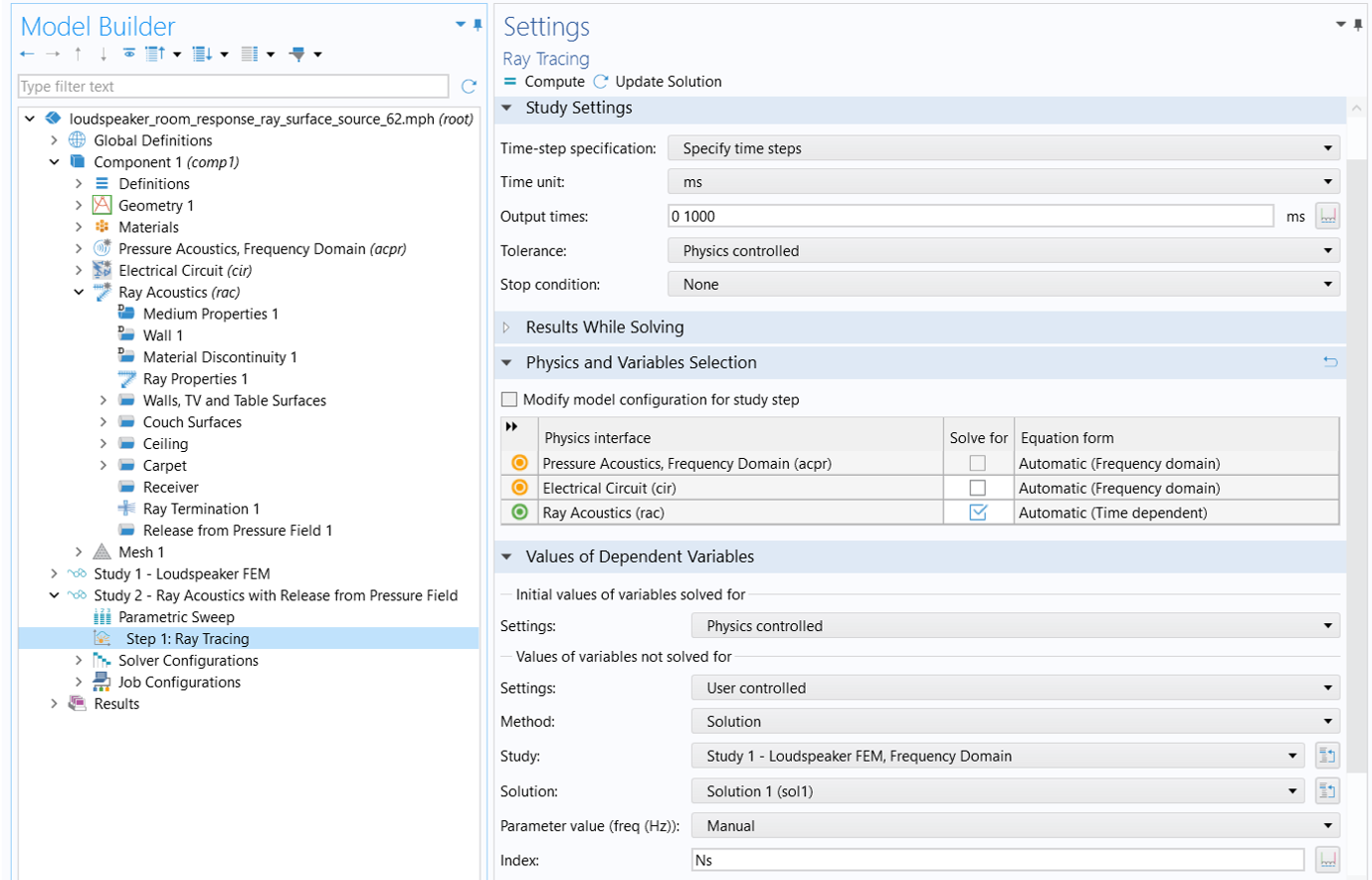
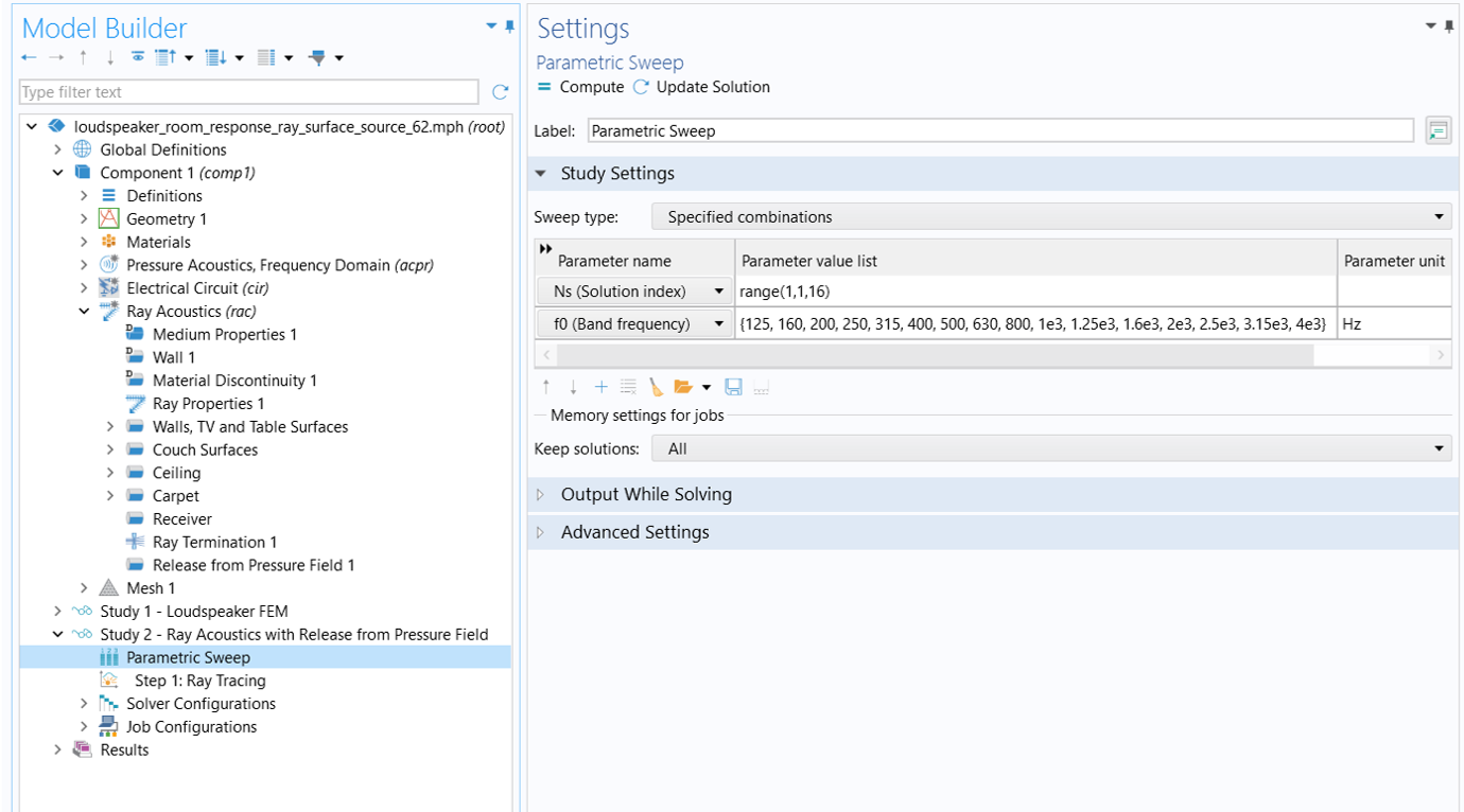
The Ray Tracing Study Settings
The study setup is identical to that in Part 3. Access to the source model solution is achieved by setting the Values of variables not solved for to use the solution from Study 1 in the Values of Dependent Variables section of the Ray Tracing study node. The solution index, Ns, is used to ensure that the correct source solution is applied for each of the 16 frequencies. The one-to-one correspondence between the solution index, Ns, and the study frequency, f0, is established in the Parametric Sweep node . For detailed explanation on study settings, please refer to the " Study Settings" sub-section under the "Ray Acoustics Model Using Release from Exterior Field Calculation" section in Part 3.
The Results
The image below shows the initial ray intensity at the time of release for the selected frequencies. As you can see, they match exactly with the intensity distribution pattern for the same frequency displayed in the source model results section.
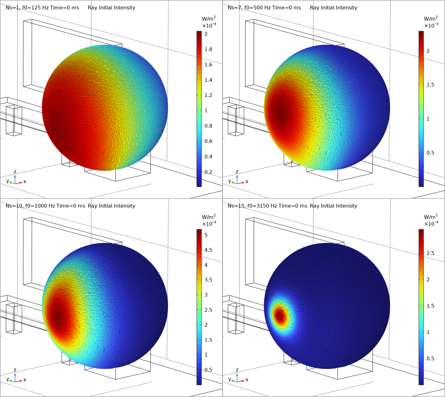 Four spheres with colored points on the surfaces indicate a different initial ray intensity for different frequencies.
The initial ray intensity for the selected frequencies.
Four spheres with colored points on the surfaces indicate a different initial ray intensity for different frequencies.
The initial ray intensity for the selected frequencies.
The images below show the ray trajectory at 8.47 ms (left), and the the sound pressure level on the surfaces at 1000 ms (right). The time is chosen for comparison with the ray trajectory at 10 ms in Part 3. Note that the release time is defined as t=0 at the release boundary, so there is a time delay (the time of flight from the point ray source in Part 3 to the release boundary used in this part) of 1.53 ms, since the radius of the release surface is 0.525 m. The color range in the legend is also set to match that used in Part 3.
 Colored dots in the room indicated the ray trajectories on the left and the surfaces are colored to show the sound pressure levels on the right.
Ray trajectories (left) and SPL plots (right) showing the ray tracing solutions for using Release from Pressure Field.
Colored dots in the room indicated the ray trajectories on the left and the surfaces are colored to show the sound pressure levels on the right.
Ray trajectories (left) and SPL plots (right) showing the ray tracing solutions for using Release from Pressure Field.
The impulse response analysis is conducted in the same manner as described in Part 3. The resulting impulse response is shown in the left image below, and its frequency spectrum is shown on the right.
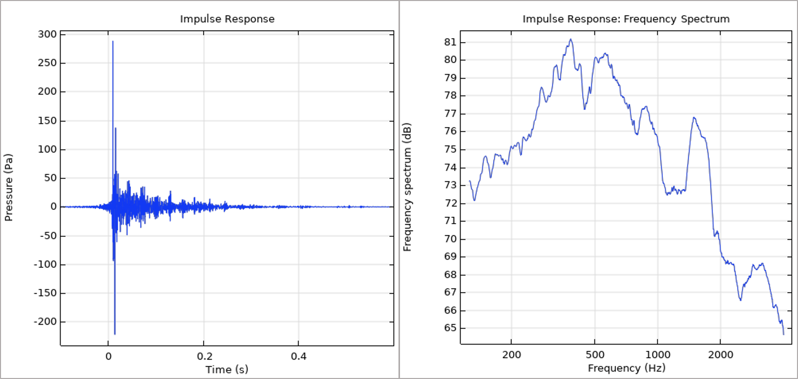 Two graphs show the pressure vs time and the frequency spectrum vs frequency with blue line plots.
Impulse response (left) and its frequency spectrum (right) calculated using the Release from Pressure Field feature.
Two graphs show the pressure vs time and the frequency spectrum vs frequency with blue line plots.
Impulse response (left) and its frequency spectrum (right) calculated using the Release from Pressure Field feature.
Envoyer des commentaires sur cette page ou contacter le support ici.