

Mixers are used for different purposes in many modern industries. If you are looking for an efficient mixer design process, you need a simulation tool that enables you to mix and match different mixer elements. With the COMSOL Multiphysics® software, you can create a mixer geometry that fits your own needs. Today, we’ll discuss modeling a laminar mixing problem with a flat-bottom mixer and two turbulent mixing problems with dished-bottom mixers that utilize the k-epsilon and k-omega turbulence models.
Mixers: A Wide Variety of Applications and Goals
Industrial mixers are a key element in many fields, from the pharmaceutical and food industries to consumer products and plastics. Further, the purpose of mixers can vary greatly. Mixers are not only used to combine elements and create homogeneous mixtures, but to also reduce the size of particles and generate chemical reactions.
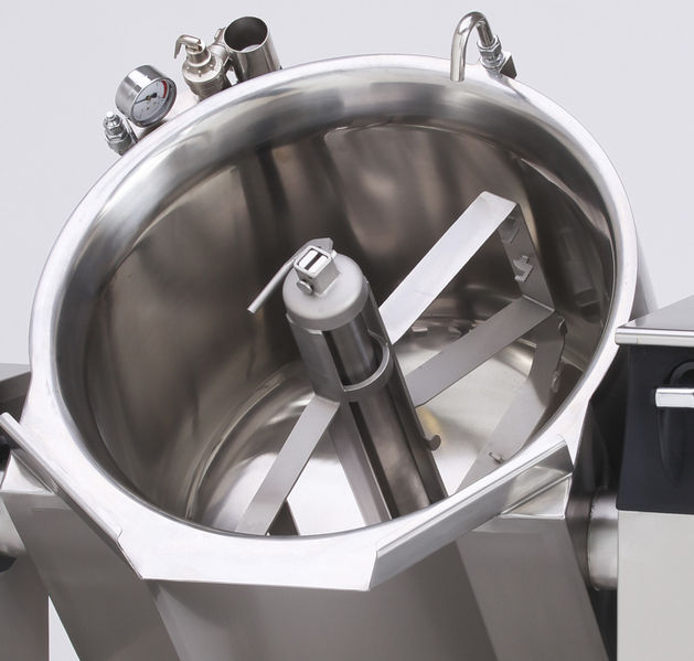
An industrial mixer. Image by Erikoinentunnus — Own work. Licensed under CC BY-SA 3.0, via Wikimedia Commons.
Mixers are required for efficient and timely production as well as for producing a uniform product quality within a batch and between batches. In some cases, mixers are required for the safe operation of systems, for example, in exothermic reactions that may create hot spots and runaway reactions (explosions) under poor mixing. With modeling, we can run inexpensive and streamlined experiments with different mixer designs in order to optimize the mixing process, avoid poor product quality, and meet safety requirements.
To resolve these issues, you can turn to COMSOL Multiphysics, which provides you with the tools for testing a wide assortment of mixers. In the next section, we’ll discuss three different mixer design examples that speak to the versatility of COMSOL Multiphysics.
Generating Three Modular Mixer Studies with COMSOL Multiphysics®
A typical batch mixer generally consists of two main components: a vessel and an impeller, both of which can vary in type and shape. Baffles can also be added to the device to improve the mixing by suppressing the bulk’s main vortex formation.
The importance of the baffles depends on the type of impeller. Radial impellers, for instance, require baffles to work. Otherwise, the solution will rotate like a merry-go-round and mixing will not be achieved. Here, the impellers will only create vertical mixing as the solution hits the walls of the vessel. Axial impellers, on the other hand, create a vertical mixing flow at the impeller, which means they do not require baffles to achieve mixing. However, axial impellers also have a radial component, so baffles can be used to increase radial mixing in axial impellers, if desired.
Let’s take a look at a mixer’s vessel, shown below, which is often modeled as either a vertical cylinder with a dish-shaped or flat bottom.
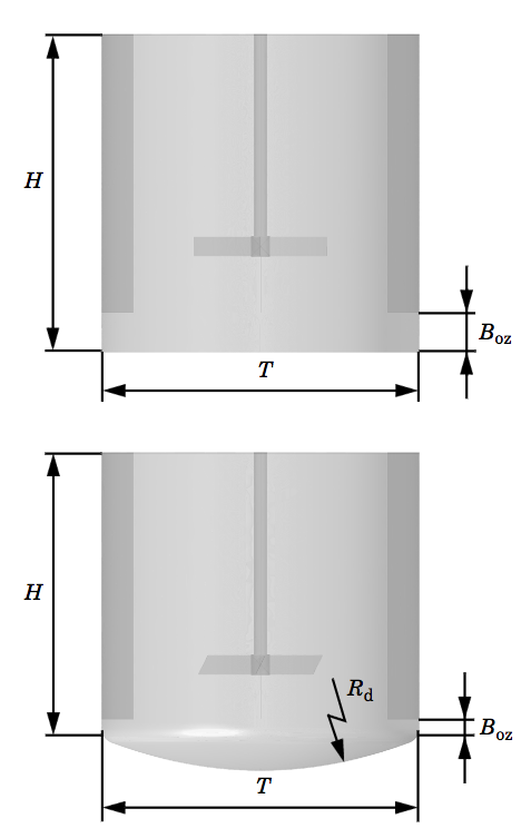
Side views of a flat-bottom mixer (above) and a dished-bottom mixer (below).
Within the vessel, the fluid is mixed by a rotating impeller. The rotation and design of the impeller determines the axial and radial direction in which the liquid is discharged. As such, impellers come in many different designs, enabling them to be used for a variety of different industrial purposes. Here, we will investigate a six-blade Rushton disc turbine, which is a radial impeller used for high-shear mixing, and a more general-purpose pitched-blade impeller, which is an axial impeller.
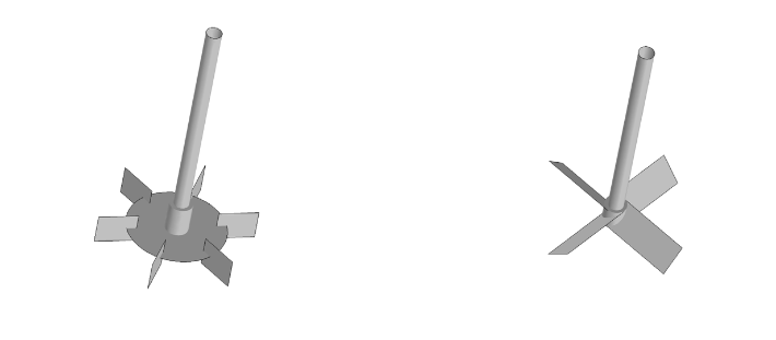
A Rushton disc turbine with six blades (left) and a pitched-blade impeller with four blades (right).
By combining these two common types of vessels with two types of impellers, we create two separate geometries (shown below) and three separate studies. All three studies use the Frozen Rotor study type and the Rotating Machinery, Fluid Flow interface.
The first study involves the laminar mixing of silicon oil in a baffled flat-bottom mixer that contains a Rushton turbine with six blades rotating at 40 rps. While we focus on the highest of three rotation rates in this example, you can easily adjust the rotation to simulate the slower rotation rates. This first example is based on a PhD thesis by M.J. Rice entitled High Resolution Simulation of Laminar and Transitional Flows in a Mixing Vessel (see Ref. 1 in the model documentation) and includes comparisons from the PhD thesis Study of Viscous and Visco-elastic Flows with Reference to Laminar Stirred Vessels by J. Hall (see Ref. 2 in the model documentation).
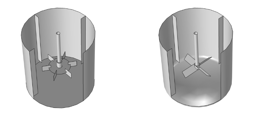
Two mixer geometries, one combining a baffled flat-bottom mixer and a Rushton turbine (left) and one with a baffled dished-bottom mixer and a four-blade pitched impeller (right).
Moving on, our next two examples deal with the turbulent mixing of water within a baffled dished-bottom mixer. This mixer contains a pitched four-blade impeller that rotates at 20 rpm. It’s possible to reduce the computational time required to solve these models by using periodicity and only simulating a quarter of the domain.
Our turbulent mixing examples enable you to explore how different models affect your results. Here, we compare a k-epsilon (k-ε) model, which has a quick convergence rate, to a k-omega (k-ω) model, which works better for flows with recirculation regions.
Comparing Results for Laminar and Turbulent Mixer Simulations
Let’s begin by looking at the velocity magnitude and in-plane velocity vectors for our three models. These results provide a general view of the circulation patterns in the mixing vessels for all three of our examples.
For our first mixer model, the laminar mixing example, we can see that the fluid is discharged radially outward by the Rushton turbine, creating two zonal vortices. The resulting compartmentalization phenomenon, which is common for radial impellers, is also displayed in our simulation results. This leads to mixing in the top and bottom vortices, albeit less intensely than inside each individual vortex.
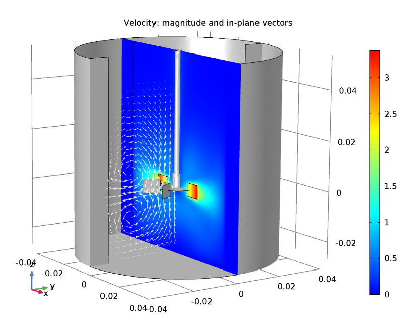
The velocity magnitude (xz-plane) and in-plane velocity vectors (yz-plane) for the laminar mixing example.
On the other hand, the velocity magnitude and vector projection for the turbulent flow k-ε model indicate that the fluid is expelled axially and radially by the pitched-blade impeller. As a result, a large zonal vortex is generated from the top to the bottom of the vessel. Additionally, a small zonal vortex appears below the impeller, which can aggregate the heavy dispersed particles in this area.
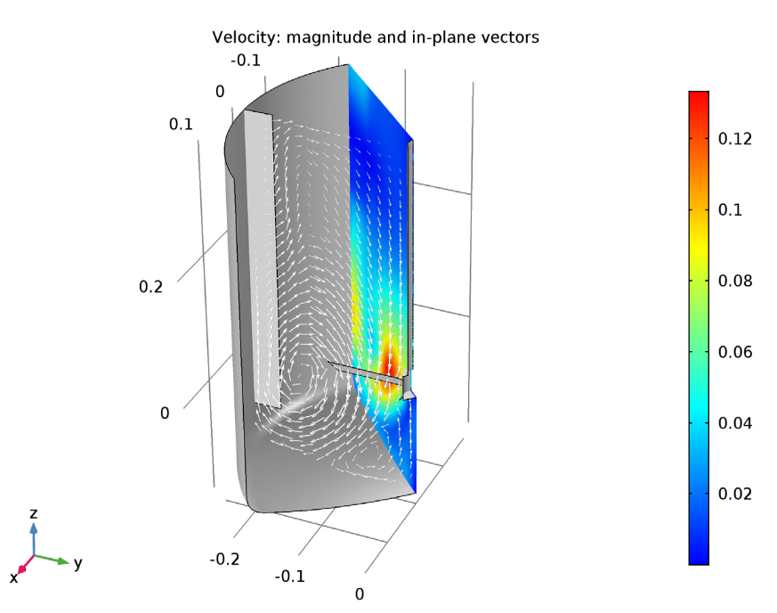
The velocity magnitude (xz-plane) and in-plane velocity vectors (yz-plane) for the k-ε turbulence model example.
The third study reveals that the turbulent flow k-ω model has a large zonal vortex, similar to the k-ε example. However, this time, the core is more vertically stretched. For its part, the smaller zonal vortex located beneath the impeller is stretched in the radial direction. Another difference lies with the torque and power draw values, which are both higher than the k-ε model. While the k-ω model is a good model to use for these types of flows, we still need to determine if its results are actually more valid than the k-ε model. Comparing simulation results to experiments is, therefore, a necessary next step.
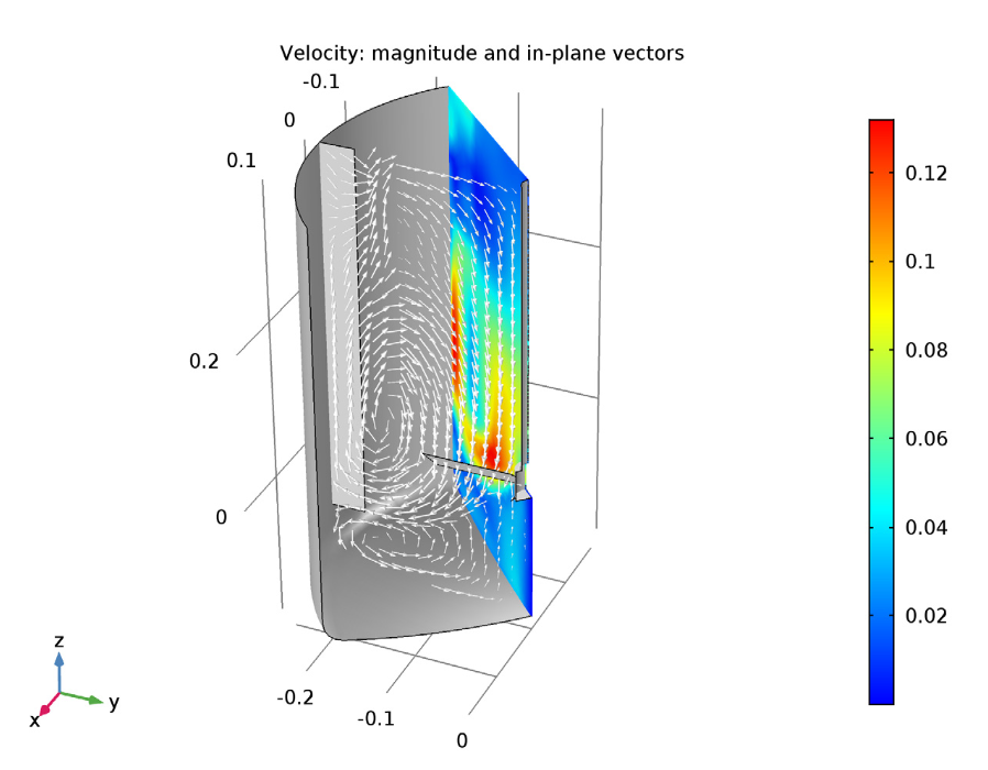
The velocity magnitude and in-plane velocity vectors for the k-ω turbulence model example.
Finally, our simulations reveal that all three examples generate good approximations for at least a few averaged flow quantities. Our results from the frozen rotor simulation for the laminar mixing study can be easily used as initial conditions for a new time-dependent study.
Modifying Mixer Geometries to Fit Your Individual Needs
It’s easy to modify the mixer geometries presented here to fit a wide assortment of mixer designs and conditions. Simply change the parameters in the supplied model to alter the types of components and properties of the geometry. For further customization, you can also add your own subsequences into the mix. With this, you can create a customized model to fit your specific application.
For more information on how to improve your mixer simulations, check out the resources in the next section.
Additional Resources to Help Your Mixer Modeling Process
- Try out the tutorial featured in this blog post: Modular Mixer-Turbulent Mixing (k-omega)
- Read a few blog posts on simulating mixers in COMSOL Multiphysics:
- Watch this in-depth archived webinar: Simulating Mixers and Non-Ideal Reactors
- Download a related tutorial: Laminar Flow in a Baffled Stirred Mixer


Comments (0)