
Since we released version 5.0 of the COMSOL Multiphysics® software, you have the ability to create simulation apps — either starting from scratch or with a demo app from the Application Library. Today, we’ll introduce you to an app that can be used for understanding and optimizing mixer design and operation for a given fluid. The exemplified app models and simulates stirred tank mixers, which are used for reactors in the fine chemical, pharmaceutical, food, and consumer products industries.
An App for Optimizing Mixer Design
In addition to the aforementioned industries, stirred batch reactors are also frequently used for lab-scale kinetic studies and when developing new processes and synthesis. In all of these processes, it’s required to obtain a relatively uniform reactor solution composition and temperature. Achieving this would allow for a reproducible and uniform product quality.
By creating an app, you can provide a user-friendly simulation environment where scientists, process designers, and process engineers can investigate the influence that vessel, impeller, and operational conditions have on the mixing efficiency and the power required to drive the impellers. We created the Mixer app to help you get started building such an app on your own.
A challenge when designing applications is getting an automatic update of geometry, physics, and mesh settings for fully parameterized geometries. It can also be difficult to include completely different geometry objects, depending on the user’s input when running the app. The Mixer app demonstrates the use of geometry parts and cumulative selection for automatic model settings.
In addition, the example also demonstrates how to build an app using COMSOL Multiphysics and how geometry parts and cumulative selections can be used to automatically set domain and boundary settings in models embedded in an application. These settings can be created automatically, even when the choices an app user makes create very diverse geometries.
The demo app can be used as a starting point for more elaborate mixer apps containing more options for the fluid flow. For example, two-phase flow and non-Newtonian flows, as well as for vessel and impeller geometries.
What the Demo App Looks Like
The annotated screenshot of the user interface (UI) below shows the 11 different types of impellers (1) that can be added to a model and the different tank types (2): dished, flat, and cone bottom, with and without baffles. The dimensions of the impellers and vessels can be set for the different types. The fluid properties and rotational speed of the impeller are selected in the Fluid Properties & Operating Conditions section (3). The Home ribbon tab (4) contains the mesh and compute buttons, which generate the numerical model and solve the model equations.
The results show the eddy diffusivity and the velocity field, both in 3D and in a vertical cut plane along the reactor (5). The cut planes can be rotated to show the results at different angles around the shaft (6). The results also give an estimate of the mixing time scale (7).

Annotated screenshot of the Mixer app.
In this specific case, the impeller is equipped with three axial impellers with c-shaped double blade sections, so-called Ekato® Intermig impellers, distributed over the length of the impeller shaft. The cut plane shows the eddy diffusivity, which is a measure of the local mixing, where red is “good” and blue is “bad”.
The 11 different types of impellers give great freedom in the creation of various impeller shapes. For example, by using hydrofoils or constant-pitched impellers in combination with cuts and fillets, you can create different propeller-type impellers.
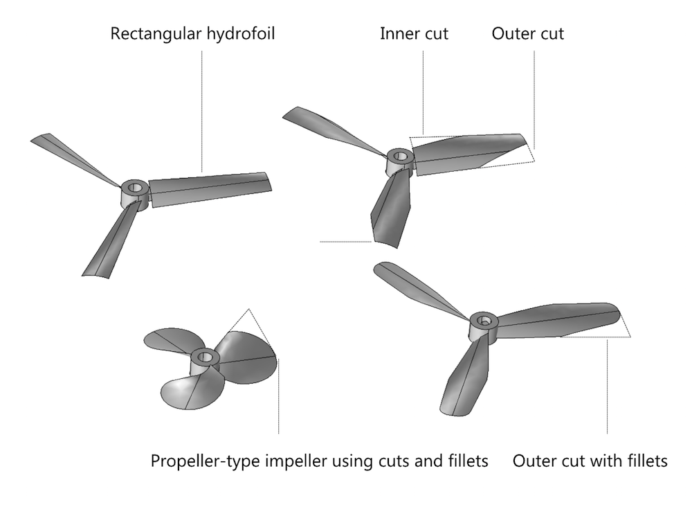
Different impeller shapes created with the hydrofoil with constant pitch impeller type, which is one of 11 available impeller types in the app.
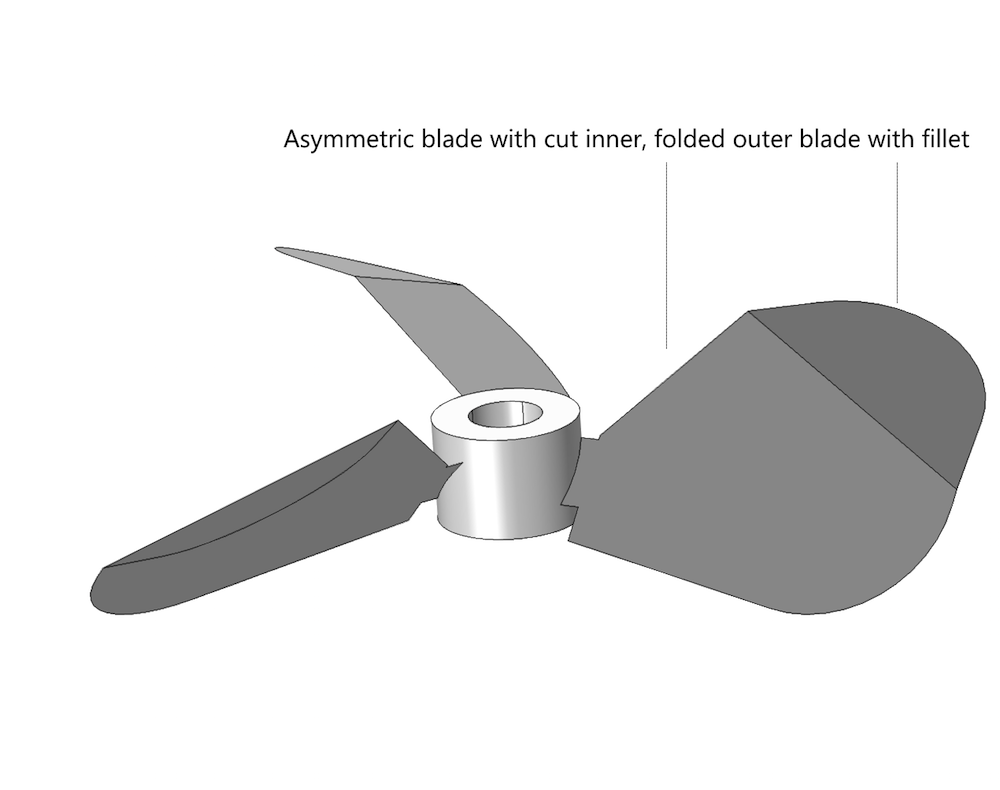
The pitched impeller with folded blades can create asymmetric blades with rounded folds using fillets.
Details of the Embedded Model
The model geometry is defined in the embedded model by a number of so-called geometry parts. For example, there are eleven different parts, one for each impeller type.
The parts are called in the main geometry sequence by the part instances (1). The part instances use parameters as input. You may compare the part instance to a function call with the input parameters as arguments. These input parameters (2) control the dimensions and the configuration of the geometry defined by the part. For example, the c-shaped double-blade axial impeller may receive parameters for the radius of the impeller and the number of blades. The geometry defined by the part may also be positioned relative to other objects in the main geometry sequence, such as relative to a work plane in the main sequence (3), for instance.
The output of the part is the geometry object (or several objects) itself together with a number of selections. An example of a selection created in a part is the Impeller Blades selection.
The selection created by the part instance may contribute to selections for domain, boundaries, edge, and point selections. For example, the Arm selection and the C-shaped blades selection both contribute to the boundary selection “Impeller Blades” (4). The “Impeller Blades” selection is referred to as a cumulative selection.
Note: We have covered cumulative selections in more detail in this blog post.

The part instance in the embedded model takes the output selections from the part and gathers them in cumulative selections according to the settings specified in its settings window.
In the same way, several impellers and impeller types can contribute to the Impeller Blades selection. When setting boundary conditions, the cumulative selections listed in the Contribute to column will be available in the list box for all boundary condition features.
The same methodology is used for the definition of the vessel and the baffles attached to the vessel wall.
By creating selections (in the geometry part) that contribute to other cumulative selections defined in the part instance, we allow for the automatic update of domain, boundary, edge, and point selections in the physics, mesh, and plot settings. A change in the geometry automatically updates the selections in all other settings, see the figure below.
The Physics that Drive the App
The physics in the model are quite straightforward. The model equations are the Navier-Stokes equations for fluid flow combined with a distributed algebraic equation, defined in every point in space, for the turbulent viscosity. The algebraic equations use the distance from no-slip walls as a variable in the equations. This is computed in the model by solving a wall distance function equation. The flow equations are solved using the frozen rotor approximation for rotating machinery.
The cumulative selections are extensively used in order to automatically update the domain settings and the boundary conditions. For example, the Rotating Interior Wall boundary condition in the Fluid Flow interface gets its selection from the Impeller Blades cumulative selection (see the figure below).
")
Screenshot detailing that the Rotating Interior Wall receives its selection from the associated “Impeller Blades” cumulative selection.
The embedded model uses a physics-controlled mesh. The mesh, which is produced automatically, includes boundary layer meshing in order to resolve the boundary layers formed along no-slip walls and rotating walls.
The solution is computed in two steps by the solver. The first step computes the wall distance, since this problem is independent of the flow field. The second step computes the solution to the Navier-Stokes equations and the turbulence equation. The turbulence equation uses the wall distance function as input.

Image showing the resulting eddy diffusivity and velocity streamlines in the Mixer app with three C-shape double blades as above but with four baffles added.
The Structure of the Application Builder UI
The figure below shows the Mixer app in the Application Builder’s Form Editor, where the user interface can be designed using drag-and-drop of different graphics and widgets selected in the ribbon menu.
The app UI consists of two areas:
- One on the left-hand side for text input and outputs with the title “Settings” in blue
- Another on the right-hand side for graphics output with the title “Graphics” in blue
")
The application UI during construction in the Application Builder.
The Application Builder screenshot above hints at the structure of the application’s UI. The form denoted main (1) is linked to the Main Window node (2) using the form reference in the Main Window settings (2). The main form contains two form collections with tabs.
The first form collection contains the general (3) and impeller_settings forms (4), with the titles General and Impeller shown in their respective tabs (5). The general and impeller_settings forms are in turn section form collections including all other forms that begin with general_ and impeller_ in the Application Builder tree. Section form collections group their member forms in sections, for example the general_tank form (6) that has Tank Type & Dimensions as the section title (6).
The second form collection in the main form contains the graphics forms (7). The graphics forms are also grouped in tabs and are the forms that begin with graphics_ in the Application Builder tree. For example, the graphics_geometry form (8) is the form with the title Geometry (9) and is shown at the top in the screenshot above.
Almost any widget contained in the forms can be linked to a command in the embedded model. For example, the Tank Type list box (10) is linked to a method that selects the tank type that will be built when the application user updates the geometry. The Update button widget (11) in the ribbon is in turn linked to the method that updates the geometry in the embedded model.
Possible Extensions
Despite its apparent complexity, the Mixer app is quite straightforward to create once the embedded model is available. The design of the geometry parts and the cumulative selections also make the embedded model relatively easy to parameterize and automate.
Future versions of the app will contain two-phase flow as well as data output for required impeller torque, flow number, and pumping capacity.
Next Step
Run the Mixer app now for inspiration and start creating your own mixer design apps with COMSOL Multiphysics.
Ekato® is a registered trademark of Ekato Holding GmBH.


Comments (1)
Andrew Ersan
June 20, 2016Hi, in comsol multiphysics there is a mixer module as a app. I want to learn in this module power that is required to drive the impellers. In below link there are two picture one is mixer_app and other one is Application_Builder_mixer. Now I have a mixer_app interface and I want to add “Required Impeller Torque” and “Required Power” in my mixer_app interface.
http://cdn.comsol.com/release/52/mixer-module/mixer_app.png
http://cdn.chemengonline.com/wp-content/uploads/2014/11/548726a5eabfa-COMSOL_5_0_Application_Builder_mixer.jpeg