Les piles à combustible sont parmi les nouvelles technologies les plus populaires dans le domaine de l’énergie propre. Elles produisent de l’électricité par le biais de réactions électrochimiques impliquant de l’hydrogène et de l’oxygène, la somme des réactions produisant une oxydation de l’hydrogène et une réduction de l’oxygène. Dit simplement, si une pile à combustible dispose d’un approvisionnement régulier en hydrogène et en oxygène, elle produira de l’électricité. En outre, le sous-produit généré par ce processus est l’eau, ce qui en fait un « combustible propre », qui ne génère pas de dioxyde de carbone ni de sous-produits toxiques.
Explorer différentes technologies de piles à combustible
Le fonctionnement optimal d’une pile à combustible implique de maintenir un équilibre entre la distribution de densité de courant dans la cellule, l’alimentation en réactifs et le profil de température. Ces aspects sont généralement étudiés à l’aide de la modélisation et de la simulation. Un modèle multiphysique pourrait également prendre en compte les éventuelles déformations structurelles dues à la dilatation thermique. Le module Fuel Cell & Electrolyzer, un produit complémentaire du logiciel COMSOL Multiphysics®, permet de concevoir et de modéliser différentes piles à combustible et d’intégrer tous ces aspects dans un seul modèle. Le logiciel offre divers couplages multiphysiques, tels que l’écoulement réactif, l’écoulement non isotherme, etc., que vous pouvez mettre en oeuvre pour obtenir une image claire du fonctionnement de la cellule dans des applications réelles. Vous pouvez également étendre ces études à des piles à combustible complètes.
Voyons quatre exemples de l’utilisation de COMSOL Multiphysics pour évaluer les différents aspects des designs de piles à combustible…
1. Pile à combustible à oxyde solide
L’électrolyte et les électrodes sont constitués d’oxydes métalliques (matériaux céramiques durs) dans une pile à combustible à oxyde solide. Les électrodes de cette cellule sont des électrodes de diffusion de gaz (GDE) poreuses, et l’électrolyte solide est placé entre elles pour former une structure en sandwich. Dans cette section, nous explorerons via la modélisation et la simulation le fonctionnement interne d’une pile à combustible à oxyde solide à l’aide du tutoriel Current Density Distribution in a Solid Oxide Fuel Cell.
Ce tutoriel peut être utilisé pour modéliser la distribution de densité de courant dans une cellule unitaire d’une pile à canaux parallèles à flux opposés. Le combustible dans cette cellule est de l’hydrogène gazeux humidifié (hydrogène et vapeur d’eau), entrant par l’anode. De l’air humidifié (vapeur d’eau, oxygène et azote) est fourni du côté cathodique.


Figure 1. La géométrie d’une cellule dans une pile à combustible à oxyde solide, incluant les plaques bipolaires (gauche). La géométrie du modèle est une cellule unitaire, incluant un canal d’air et un canal d’hydrogène (droite). La plaque bipolaire est supposée être à potentiel électrique constant et n’est pas incluse dans le modèle. A la place, le potentiel électrique est défini comme condition aux limites aux surfaces de contact entre les GDE et les plaques bipolaires.
Ce modèle inclut un couplage complet entre:
- Les bilans de masse à l’anode et à la cathode
- L’écoulement dans les canaux de gaz
- L’écoulement de gaz dans les électrodes poreuses
- Le bilan du courant ionique transporté par l’ion oxyde
- Un bilan de courant électronique
- Les réactions de transfert de charge (réactions électrochimiques) à l’anode et à la cathode
Ce modèle, qui constitue un véritable problème multiphysique, implique plusieurs interfaces physiques décrivant les processus et phénomènes se produisant dans la cellule. Les équations de diffusion et convection de Maxwell–Stefan décrivent le transport de matière dans la phase gazeuse, résolues avec l’interface Pile à combustible à hydrogène. L’écoulement à travers les canaux ouverts est défini par les équations de Navier–Stokes compressibles, tandis que les équations de Brinkman décrivent la vitesse d’écoulement à l’intérieur des électrodes poreuses. Le bilan de courant dans l’électrolyte, l’électrolyte poreux et les électrodes est défini en utilisant la théorie des électrodes poreuses, couplant la concentration locale dans les GDE avec l’équation de Nernst pour la thermodynamique et les expressions de Butler–Volmer pour la cinétique des réactions de transfert de charge (cinétique des électrodes).
Il est intéressant d’étudier dans ce modèle les relations entre:
- La largeur des canaux
- L’épaisseur des électrodes
- La conductivité de l’électrolyte (y compris l’électrolyte poreux)
- La conductivité des électrodes
- La longueur de la cellule
- La composition du gaz et le débit d’alimentation en gaz
Ces paramètres de conception et de fonctionnement déterminent la performance de la cellule sous différentes charges. Le modèle est entièrement paramétré, ce qui signifie que vous pouvez exécuter les simulations pour différentes valeurs des paramètres ci-dessus afin de comprendre et d’étudier le comportement de la cellule. Vous pouvez avoir un aperçu des résultats de ce modèle dans la section ci-dessous, puis comprendre en détail comment le construire en consultant le fichier MPH associé et les instructions PDF dans la Bibliothèque d’applications.
Résultats de la modélisation
De gauche à droite, les graphiques de la Figure 2 montrent la fraction molaire d’hydrogène à l’anode, la fraction molaire d’oxygène à la cathode et la densité de courant dans l’électrolyte. Le modèle montre que l’alimentation en air limite la performance de la cellule, entraînant une densité de courant élevée à l’entrée d’air et une densité de courant faible à la sortie d’air. De plus, nous pouvons voir que la densité de courant est légèrement plus élevée au milieu des canaux par rapport aux bords, où le collecteur de courant et les surfaces de contact de l’alimentation gênent le transport du gaz.


Figure 2. Graphiques montrant la fraction molaire d’hydrogène à l’anode (gauche) et la fraction molaire d’oxygène à la cathode (milieu) à une tension de cellule de 0.6 V, avec la composition représentée dans les canaux de gaz et les électrodes de diffusion de gaz. La distribution de la densité de courant dans l’électrolyte (droite) montre que l’alimentation en air limite la performance de la cellule, entraînant une densité de courant élevée à l’entrée d’air.
La Figure 3 montre que la puissance maximale dans les conditions de fonctionnement de la Figure 2 se situe à une densité de courant légèrement inférieure à 1800 A/m2 (graphique de gauche ci-dessous), ce qui correspond à une puissance maximale légèrement inférieure à 1150 W/m2. Si le débit d’air augmente, la densité de puissance maximale passe à 1300 W/m2 (graphique de droite ci-dessous). Si nous devions tracer la distribution de la densité de courant dans l’électrolyte, nous verrions qu’elle est beaucoup plus uniforme. Cependant, cette performance accrue doit être mise en regard avec la puissance requise par la pompe à air, qui doit fournir une pression 50% plus élevée.


Figure 3. Courbes de polarisation et de densité de puissance à une pression d’entrée d’air de 6 bars (à gauche), montrant une puissance maximale juste en dessous de 1150 W/m2 pour une densité de courant d’environ 1800 A/m2. L’augmentation du débit d’air en élevant la pression d’entrée à 9 bars (à droite) déplace le maximum vers une densité de courant plus élevée (2200 A/m2) ainsi qu’une densité de puissance plus élevée (1300 W/m2).
2. Pile à combustible PEM basse température
Les piles à combustible à membrane échangeuse de protons (PEM) utilisent une membrane polymère comme électrolyte, généralement avec une teneur en eau relativement élevée durant son fonctionnement. Dans le tutoriel Low-Temperature PEM Fuel Cell with Serpentine Flow Field , l’assemblage électrode-membrane (MEA) — composé de la membrane et des électrodes à diffusion de gaz (GDE) — est pris en sandwich entre des plaques bipolaires, qui comprennent des canaux de gaz en forme de serpentin. Dans la géométrie ci-dessous, les canaux d’air avec leurs entrées sont situés au-dessus du MEA, tandis que les canaux d’hydrogène sont situés en dessous du MEA.
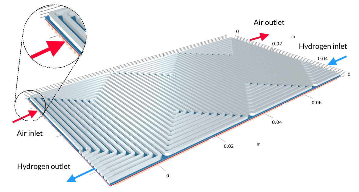
Figure 4. La géométrie du modèle de pile à combustible PEM.
La pile PEM produit de l’eau à la cathode, en raison de la réaction d’oxydation de l’hydrogène à l’anode (électrode négative) et de la réaction de réduction de l’oxygène à la cathode (électrode positive). L’eau produite peut traverser la membrane et atteindre le côté anode. Si l’eau n’est pas évacuée efficacement depuis la GDE de la cathode, les pores de l’électrode sont noyés (flooding), bloquant l’apport en oxygène et provoquant une chute significative des performances. À l’inverse, si la membrane et l’électrolyte poreux sont trop secs, la conductivité ohmique de l’électrolyte diminue. La gestion de l’eau est donc un facteur crucial dans le fonctionnement d’une pile à combustible PEM.
Ce modèle résout:
- Les bilans de charge et les équations de transport de masse dans les électrodes de diffusion de gaz et la membrane électrolytique
- Les équations d’écoulement dans la phase gazeuse de chaque côté de la membrane
- Le transport de l’eau dans la membrane par diffusion (perméation) et migration (traînée électro-osmotique)
- Les réactions de transfert de charge (réactions électrochimiques) aux électrodes
Les aspects clés à étudier avec ce modèle incluent:
- L’impact du motif en serpentin
- Les dimensions de la section transversale des canaux
- La largeur de la surface de contact entre la plaque bipolaire et les électrodes
- Les dimensions du MEA
- Les propriétés des matériaux de tous les composants de la cellule
Tous ces aspects peuvent être étudiés sous différentes conditions de fonctionnement (débits de gaz et charge). Le modèle peut également être utilisé pour optimiser la conception de la pile pour un débit de gaz et une charge donnés. Un aperçu des résultats de modélisation est présenté ci-dessous; les instructions détaillées de construction du modèle peuvent être téléchargées ici.
Résultats de la modélisation
Le modèle calcule la composition des gaz dans les GDE et les canaux respectifs, comme le montre la Figure 5. Ces graphiques montrent une diminution nettement plus importante de l’oxygène que de l’hydrogène. Cette diminution se produit sur toute l’épaisseur de la GDE, principalement en raison de la plus faible diffusivité de l’oxygène. Comme le flux d’air et le flux d’hydrogène sont en flux opposés, les deux gaz réactifs sont appauvris aux des extrémités des plaques bipolaires, de manière opposée.


Figure 5. Graphiques de la fraction molaire d’oxygène (gauche) et d’hydrogène (droite).
L’analyse de l’activité de l’eau dans le canal d’hydrogène et dans la membrane montre une activité plus élevée près de l’entrée d’air. La proportion d’oxygène est élevée dans la phase gazeuse à cet endroit, ce qui entraîne une densité de courant locale plus élevée, le taux de réaction étant limité par le transport de l’oxygène. Nous pouvons également constater que la conductivité de la membrane est plus importante là où l’activité de l’eau est élevée, ce qui a un impact sur la distribution de la densité de courant dans la cellule. La teneur en oxygène et en eau augmente la densité de courant jusqu’à ce que la proportion d’eau liquide dans la GDE cathodique commence à faire obstacle au transport du gaz.


Figure 6. Graphiques de l’humidité relative dans les canaux (gauche) et de l’activité de l’eau dans la membrane (droite).
3. Pile à combustible PEM non-isotherme
Avec le tutoriel Nonisothermal PEM Fuel Cell, nous pouvons modéliser les réactions électrochimiques couplées, les écoulements fluides, le transfert de chaleur, ainsi que le transport de charges et d’espèces dans une pile à combustible PEM. Dans ce tutoriel, la cellule comprend un assemblage membrane-électrolyte pris en sandwich entre des couches de diffusion de gaz (GDL), qui servent d’électrodes. Les couches actives des électrodes sont modélisées comme des surfaces, c’est-à-dire en négligeant leur épaisseur géométrique. (L’épaisseur de la couche active est un paramètre, mais elle n’est pas représentée comme une épaisseur dans la géométrie du modèle, ce qui signifie que la composition gazeuse et le potentiel électrique sont constants le long de l’épaisseur des couches actives.) Les canaux d’hydrogène sont formés par une plaque ondulée qui sert également de collecteur de courant en contact avec l’anode. Des canaux de refroidissement, remplis d’eau liquide, sont disposés de l’autre côté des canaux d’hydrogène. Le compartiment à air est formé par un collecteur de courant à mailles déployées qui sépare la cathode d’une plaque métallique plate. Cette dernière, placée au-dessus de la maille déployée, sert de plaque bipolaire. Elle sépare également le compartiment cathodique des canaux de refroidissement de la cellule adjacente, qui serait située au-dessus de la cellule modélisée dans une pile.
Notez que la figure 7 inclut deux cellules unitaires dans la largeur, et contient donc deux canaux d’hydrogène. En raison de la symétrie, nous n’aurions besoin de modéliser qu’un quart de cette géométrie. Cependant, comme de tels résultats sont difficiles à interpréter — et puisque les équations du modèle peuvent être résolues en quelques minutes — nous pouvons utiliser une géométrie plus grande que nécessaire.
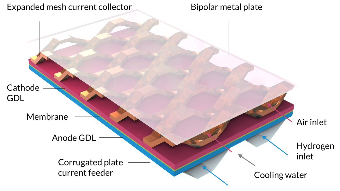
Figure 7. Géométrie du tutoriel Nonisothermal PEM Fuel Cell
Les entrées pour les flux d’air et d’hydrogène humidifiés, ainsi que pour le fluide de refroidissement liquide, sont représentées sur le côté droit de la figure.
L’eau liquide de refroidissement est décrite à l’aide des équations de Navier–Stokes pour l’écoulement laminaire avec l’interface Ecoulement monophasique, tandis que la température de la pile est définie et résolue à l’aide de l’interface Transfert de chaleur. Pour comprendre le fonctionnement global de la cellule — tenant compte de l’écoulement, du transport d’espèces chimiques, des réactions électrochimiques et du transfert thermique à travers la pile — il est nécessaire d’inclure différents phénomènes multiphysiques, qui sont définis à l’aide des noeuds multiphysiques suivants dans le modèle: Ecoulement réactif, Chauffage électrochimique, and Ecoulement non-isotherme.
Il est intéressant d’étudier l’impact de la structure en maille déployée utilisée dans le canal d’air. L’objectif de cette structure est de créer un champ d’écoulement perpendiculaire à la MEA. Cela permet l’apport d’oxygène et l’évacuation de l’eau. Les performances de la pile à combustible peuvent varier en fonction des paramètres régissant la géométrie de la maille déployée. Ces derniers peuvent influencer la relation entre le contact du collecteur de courant avec l’électrode et la surface disponible pour le transport de masse, notamment l’évacuation de l’eau. Le modèle permet d’optimiser la structure pour des conditions de fonctionnement et une charge données. Un aperçu des résultats de ce modèle est présenté ci-dessous. Pour apprendre à le construire vous-même, téléchargez la documentation PDF et le fichier MPH depuis la Bibliothèque d’applications.
Résultats de la modélisation
À gauche, le graphique ci-dessous montre la densité de courant électrolytique de la membrane, où la densité de courant augmente vers la sortie. Cela est dû à la conductivité de la membrane, qui augmente avec la teneur en eau du fait de la production d’eau. Si nous regardons la teneur en eau de la membrane, nous pouvons voir que l’eau s’accumule sous les zones de contact entre le collecteur de courant et la cathode, où la densité de courant est également élevée. Cela pourrait éventuellement devenir problématique si l’eau venait à noyer la cathode, empêchant ainsi le transport de l’oxygène. Supposons que nous allongions la pile en rendant les canaux d’hydrogène deux fois plus longs tout en maintenant constantes les conditions de fonctionnement. Dans ce cas, nous observerions une diminution spectaculaire de la densité de courant le long des canaux, car la réaction de réduction de l’oxygène serait ralentie en raison des limitations liées au transport de matière.

")
Figure 8. La densité de courant de l’électrolyte à travers la membrane (à gauche) et l’humidité relative de la membrane (à droite) pour une tension de cellule de 0.5 V.
Avec ce modèle, nous pouvons également observer la fraction molaire d’oxygène et la fraction molaire de vapeur d’eau dans un mélange gazeux cathodique. Les niveaux d’oxygène diminuent à mesure que l’on se rapproche de la sortie, tandis que les niveaux d’eau augmentent.


Figure 9. Graphiques représentant la fraction molaire d’oxygène (à gauche) et la fraction molaire d’hydrogène (à droite).
On peut également examiner le profil de température sur l’ensemble de la cellule et dans le canal de refroidissement. Les températures les plus élevées sont observées dans le MEA, ce qui est logique car c’est là que se trouvent les sources de chaleur liées à l’effet Joule et aux pertes d’activation.
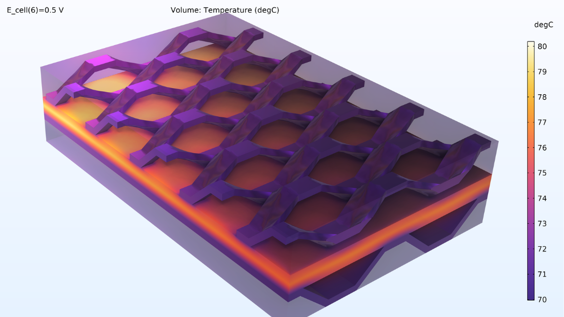
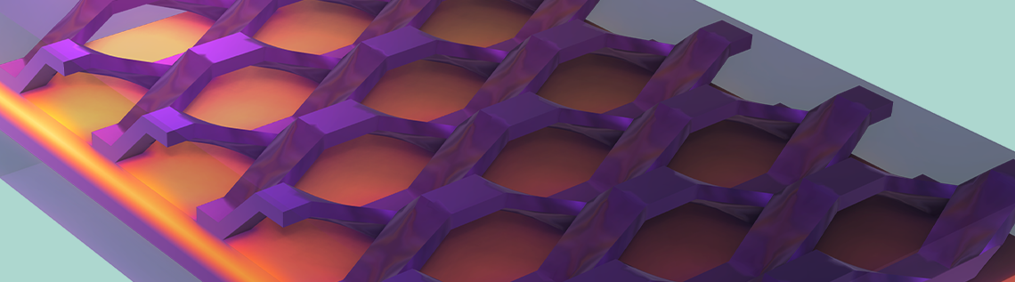
Figure 10. Répartition de la température dans la cellule.
La dissipation de puissance dans la cellule est illustrée par la figure 11. Ce graphique montre la répartition de la production de chaleur dans la cellule. Nous voyons que la source de chaleur la plus importante se trouve dans la membrane, en raison de sa faible conductivité. De plus, nous pouvons voir une génération importante de chaleur à l’endroit où la maille déployée est en contact avec la cathode. Ici, la conductivité de l’électrode est relativement faible (comparée à celle des collecteurs de courant), tandis que la densité de courant est élevée.
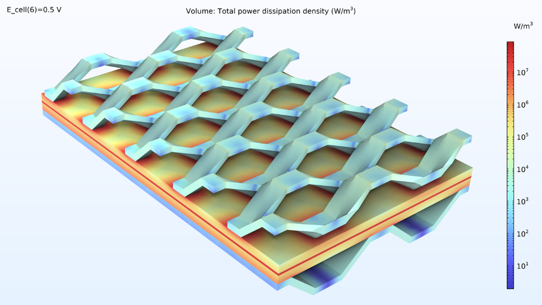
Figure 11. Représentation logarithmique des sources de chaleur dans le MEA, l’alimentation de courant et le collecteur de courant.
Enfin, nous pouvons générer une courbe de polarisation de la cellule montrant la tension de la cellule en fonction de la densité de courant moyenne (courant par unité de surface de la membrane). La diminution significative de la tension de cellule à faible densité de courant est due aux surtensions d’activation, principalement à la cathode. Une région linéaire dominée par les pertes ohmiques se dessine ensuite à des densités de courant légèrement plus élevées. Nous observons une légère augmentation des pertes à haute densité de courant, où la courbe s’incurve légèrement vers le bas en raison de la résistance liée au transport de masse.
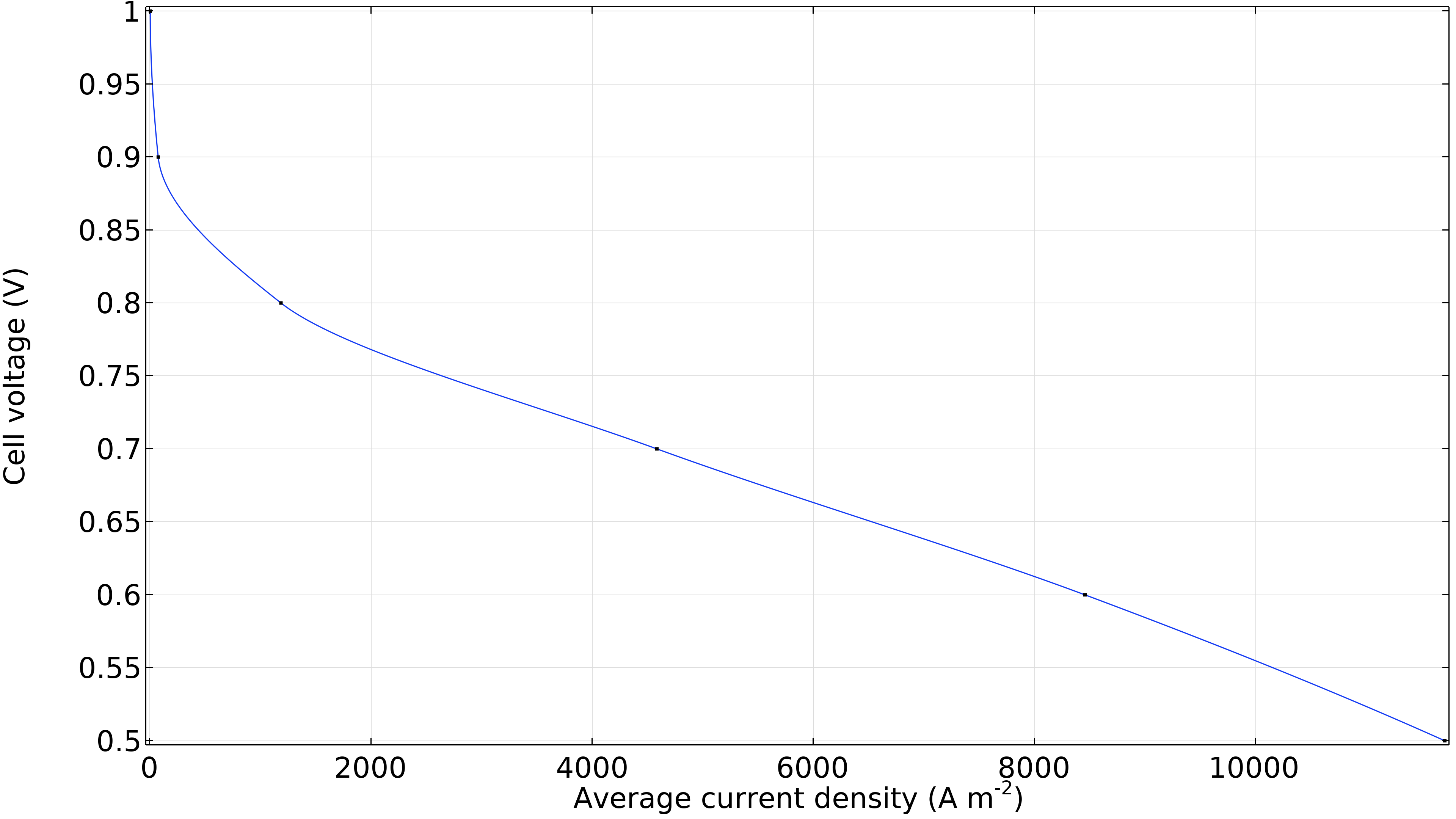
Figure 12. Courbe de polarisation montrant la tension de la cellule en fonction de la densité de courant moyenne.
4. Refroidissement d’un stack de pile à combustible
Le tutoriel Fuel Cell Stack Cooling, introduit avec la version 6.1 de COMSOL Multiphysics, peut être utilisé pour évaluer la gestion thermique d’un empilement de piles à combustible PEM constitué de cinq cellules et cinq MEA entre deux plaques terminales. Ce type d’analyse est important car une répartition inégale de la température au sein des cellules d’un empilement peut entraîner une condensation non uniforme de la vapeur d’eau et une variation indésirable des performances d’une cellule à l’autre.
Dans cet exemple, des plaques bipolaires transportant un fluide de refroidissement sont intercalées dans l’empilement. L’image de gauche montre la cellule unitaire, qui est répétée pour construire la géométrie du modèle. Quant aux images du milieu et de droite, elles montrent la géométrie finale du modèle, construite en empilant cinq cellules unitaires entre deux blocs métalliques.


Figure 13. Ici, nous pouvons voir la cellule unitaire de répétition (à gauche) ainsi qu’une vue de l’empilement de 5 cellules unitaires montrant la forme des canaux d’oxygène (au milieu) et des canaux d’hydrogène (à droite). Les plaques métalliques contenant les canaux d’air et d’hydrogène, représentées en rose et en bleu sur la figure de gauche, sont soudées dos à dos dans l’empilement. En raison du motif des canaux, un espace est laissé entre les soudures, formant les canaux d’écoulement pour l’eau de refroidissement. Les plaques terminales maintiennent la structure et appliquent une pression afin d’assurer un contact optimal entre les plaques bipolaires et le MEA.
Le modèle définit les équations pour:
- La température
- Les potentiels dans les électrodes et l’électrolyte
- Le transport d’espèces réactives dans chacun des compartiments gazeux
- Les champs de pression et d’écoulement dans les compartiments d’écoulement gazeux et liquide
- Les cinétiques électrochimiques dans les couches actives du MEA
Dans ce modèle, il est intéressant d’étudier les variations de composition, de température et de distribution de la densité de courant pouvant apparaître dans la pile. Ces aspects dépendent de la géométrie des plaques bipolaires et des MEA. Ils peuvent également dépendre du nombre de cellules incluses dans l’empilement. Le modèle permet de traiter la géométrie des canaux gazeux à l’aide d’une approche de milieu poreux, avec des propriétés anisotropes reflétant la structure des canaux gazeux. En comparant une telle approche avec la description complète des canaux gazeux, nous pouvons en vérifier la précision. L’avantage de cette approche est qu’elle offre une bonne précision (selon l’objectif) tout en réduisant considérablement le coût de calcul (temps CPU et mémoire nécessaire).
Vous trouverez ci-dessous un aperçu des résultats issus de ce modèle. Pour apprendre à le construire vous-même, téléchargez la documentation PDF et le fichier MPH dans la Bibliothèque d’applications.
Résultats de la modélisation
La figure 14 montre la distribution de la densité de courant dans la membrane entre les électrodes. L’apport en air semble contrôler la vitesse de transfert de charge, ce qui entraîne une densité de courant plus élevée à l’entrée du canal d’air et plus faible à la sortie. De plus, la distribution de densité de courant est presque identique en haut, au centre et en bas de l’empilement.


Figure 14. Densité de courant entre les électrodes dans la membrane de la cellule supérieure (à gauche), de la cellule centrale (au milieu) et de la cellule inférieure (à droite).
La figure 15 montre les fractions molaires d’hydrogène et d’oxygène dans les canaux gazeux et les électrodes poreuses de la cellule supérieure. Comme prévu, la distribution de densité de courant ci-dessus reflète le profil de la fraction molaire d’oxygène. Il convient de noter que l’oxygène est épuisé dans une bien plus grande mesure que l’hydrogène. De plus, la fraction molaire d’oxygène diminue progressivement sur toute l’épaisseur de la cathode, tandis que celle de l’hydrogène reste pratiquement constante sur toute l’épaisseur de l’anode.


Figure 15. Fraction molaire d’hydrogène (à gauche) et fraction molaire d’oxygène (à droite) dans la cellule supérieure de l’empilement.
La figure 16 montre la température dans la cellule supérieure de l’empilement, et plus particulièrement dans les canaux gazeux et l’électrode de la cathode; la membrane; les canaux et l’électrode de l’anode, représentés de droite à gauche dans les légendes colorées. La température est plus élevée dans la membrane, ce qui est attendu puisque la membrane présente une conductivité électrique et thermique plus faible. De plus, la température augmente dans la direction de l’eau de refroidissement, ce qui est également attendu.
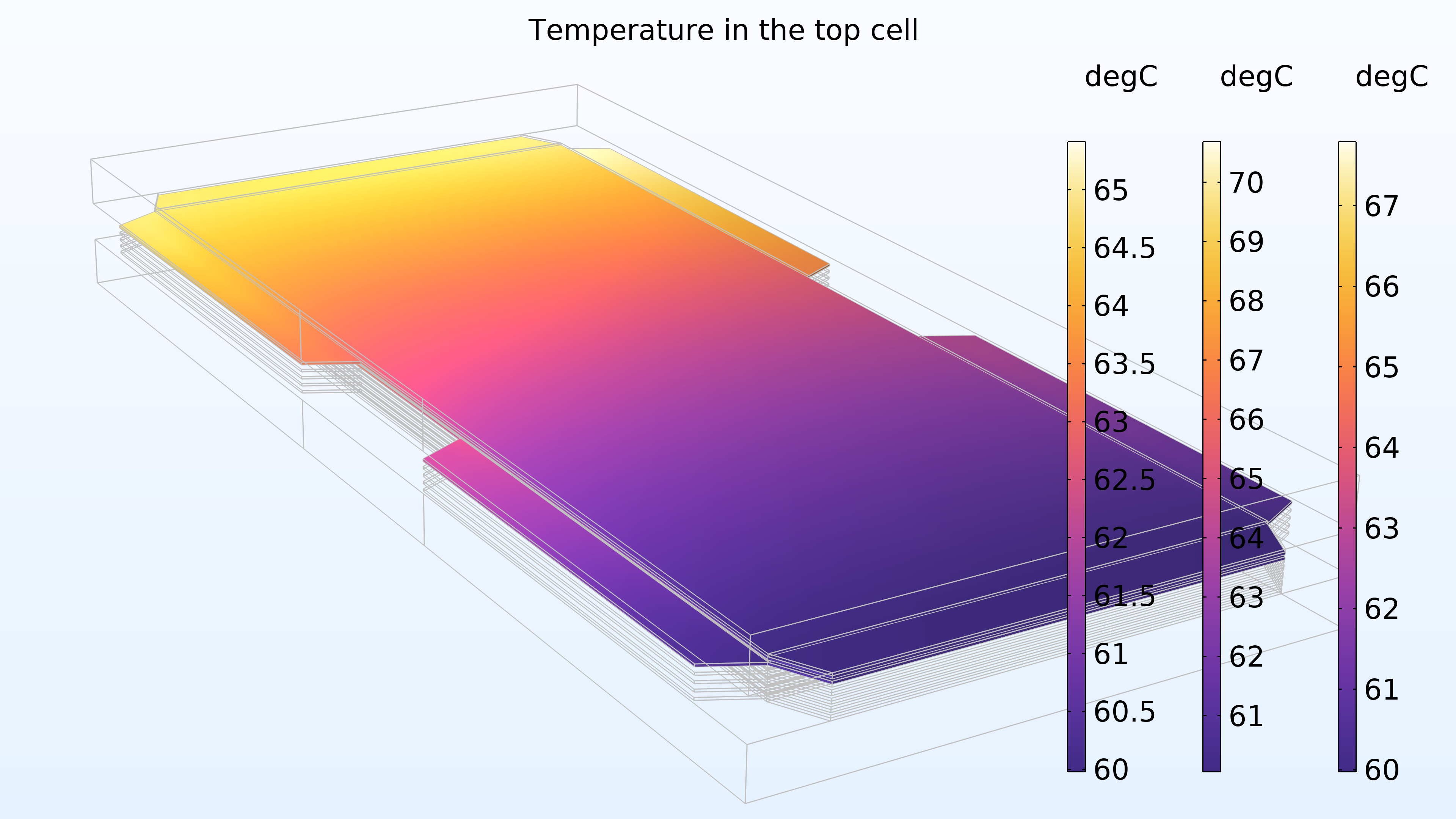
Figure 16. La température dans la cellule supérieure de l’empilement.
La figure 17 montre la température dans l’empilement. La température la plus élevée est obtenue dans la membrane de la cellule centrale. Cet emplacement est le plus éloigné des plaques terminales, qui contribuent au refroidissement. Les canaux de refroidissement dans les plaques bipolaires contribuent également au refroidissement. De plus, on peut voir que la distribution de température est identique dans les deux plaques terminales.
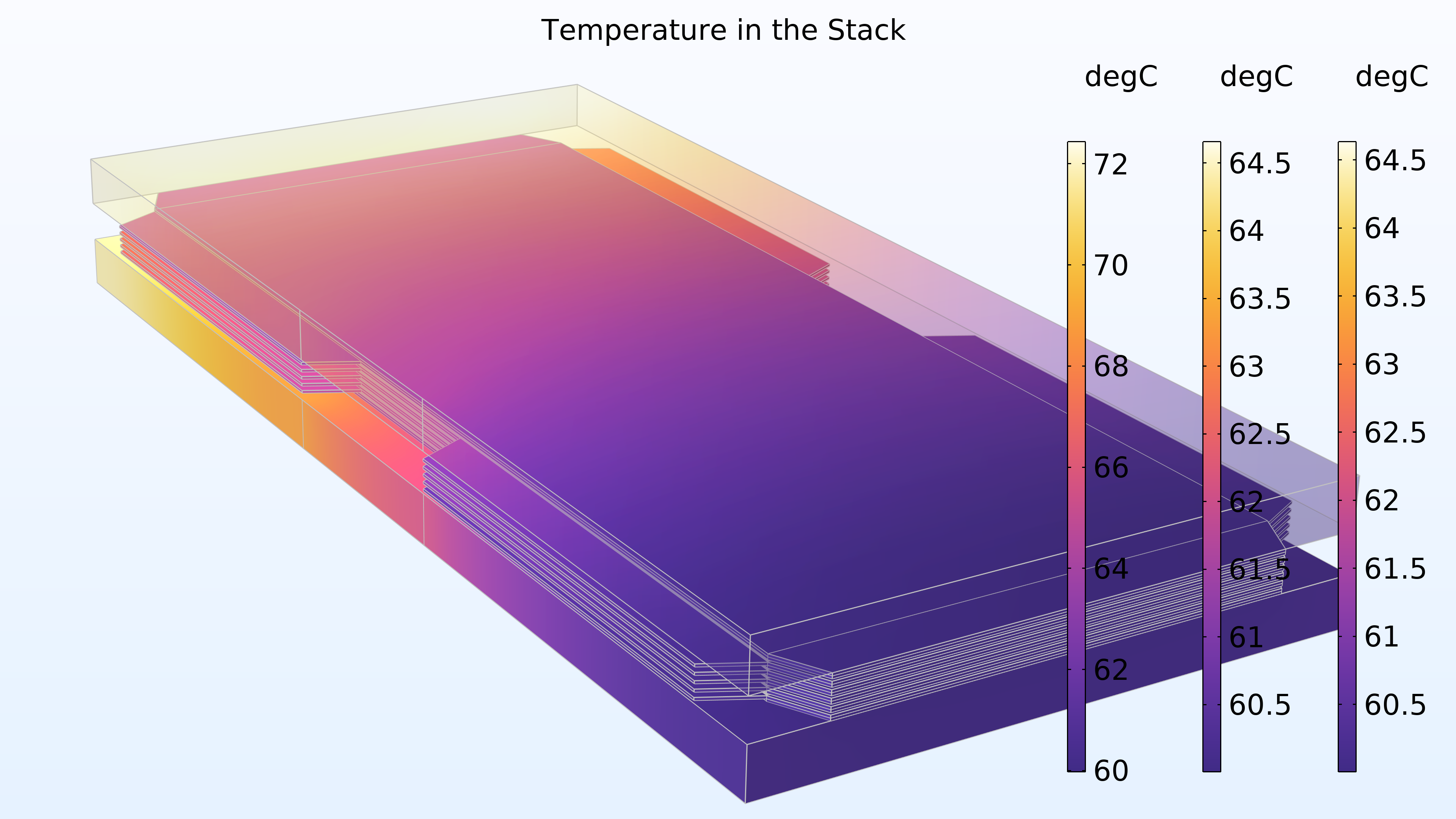
Figure 17. Température dans l’empilement. Les légendes colorées de droite et du milieu correspondent aux plaques terminales, tandis que la légende colorée de gauche correspond aux cellules.
Le modèle présente une légère variation sur la hauteur de l’empilement. Celle-ci évoluerait si nous empilions davantage de cellules, ce qui entraînerait un épuisement de l’oxygène ou de l’hydrogène sur toute la hauteur des cellules, avec également des variations dans les canaux de gaz du collecteur.
Prochaines étapes
Ce ne sont là que quelques exemples illustrant les possibilités d’utilisation de la modélisation et de la simulation dans le développement des piles à combustible, mais il en existe bien d’autres. En faisant appel à la simulation pour mieux comprendre le fonctionnement des piles à combustible, les ingénieurs peuvent continuer à améliorer leur rendement global, leur puissance et leur fiabilité.
Notez que tous les exemples présentés ici sont typiquement construits à l’aide du module Fuel Cell & Electrolyzer. Pour en savoir plus sur ce module, qui peut être utilisé pour modéliser des piles à combustible à hydrogène, des électrolyseurs industriels et bien plus encore, cliquez sur le bouton ci-dessous !

Commentaires (0)