AC/DC Module Updates
For users of the AC/DC Module, COMSOL Multiphysics® version 5.3 brings a new Electrostatics, Boundary Elements physics interface, a new Stationary Source Sweep study step, and several new tutorial models. Review all of the AC/DC Module updates in more detail below.
New Physics Interface: Electrostatics, Boundary Elements
The new Electrostatics, Boundary Elements interface has been developed for building and running models that are not well suited for the finite element method (FEM). The formulation is based on the boundary element method (BEM). The physics interface, available in 2D and 3D, solves Laplace's equation for the electric potential using the scalar electric potential as the dependent variable. This new interface can be used as an alternative to the Electrostatics interface for computing the potential distribution in dielectrics, and is particularly convenient for structures that are difficult to mesh. Note that the electric potential distribution on the boundaries must be explicitly defined, so you need constant material data within the domains.
The Electrostatics, Boundary Elements interface can also be combined with the finite-element-based Electrostatics interface, using the Boundary Electric Potential Coupling multiphysics node. As an example, you could use a combination of the two interfaces to include the effects of an infinite space instead of using the Infinite Element Domain feature.
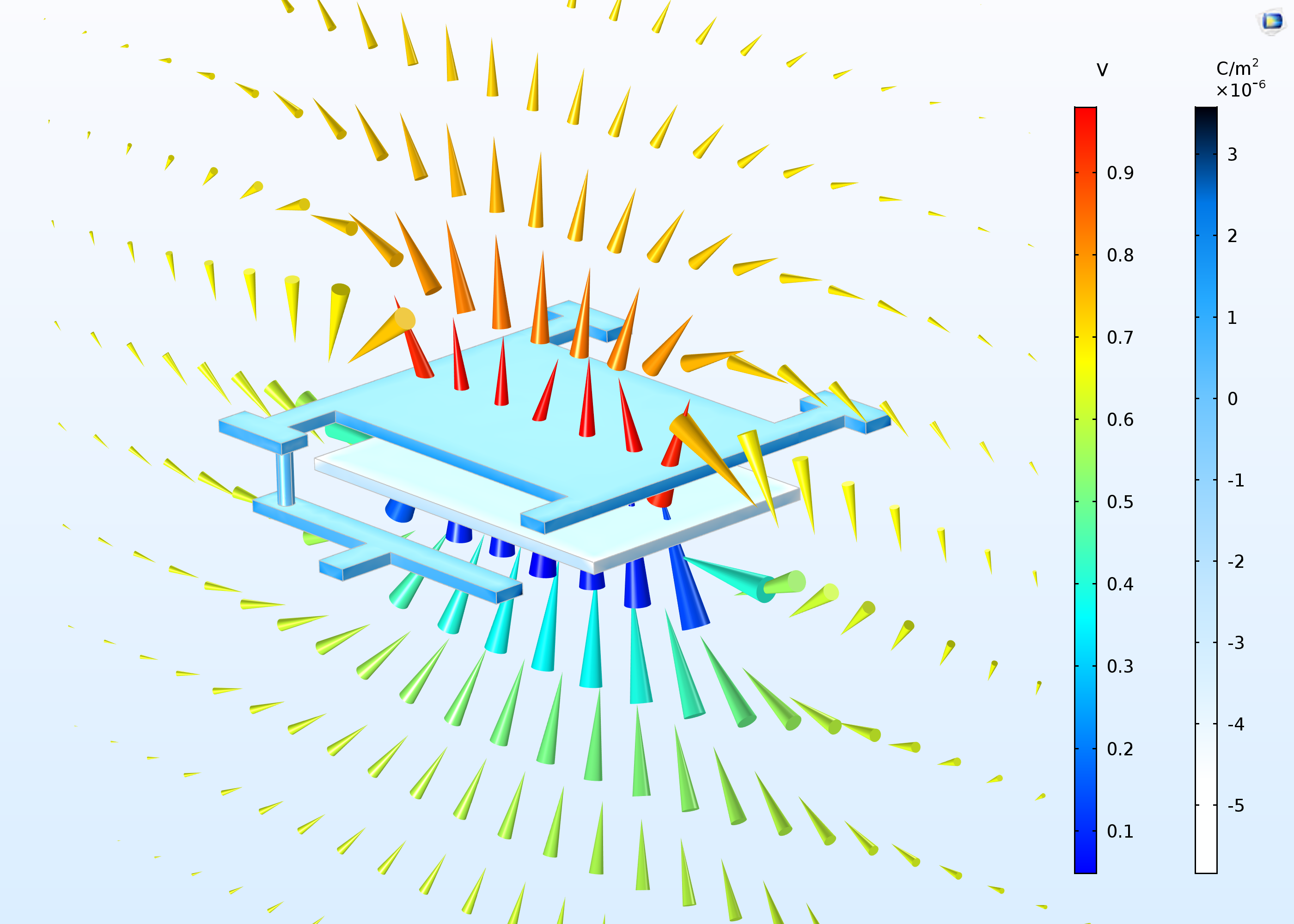 The electrostatic behavior of a tunable capacitor modeled using boundary elements. The electric field and potential are shown as an arrow plot, while the induced surface charge density is plotted on the electrode surfaces. Using the boundary element method for this simulation negates the need for defining a finite modeling domain and boundary as well as meshing the thin volume of the capacitor.
Application Library path for an example using the Electrostatics, Boundary Elements interface:
ACDC_Module/Capacitive_Devices/capacitor_tunable
New Study Step: Stationary Source Sweep
A new Stationary Source Sweep custom study is available for faster calculation of lumped parameters in the Electrostatics, Electric Currents and Electrostatics, Boundary Elements interfaces. For direct solvers, it reuses the LU decomposition of the system matrix, making it several times faster than the previous port sweep implementation. The speed when using an iterative solver has also been improved.
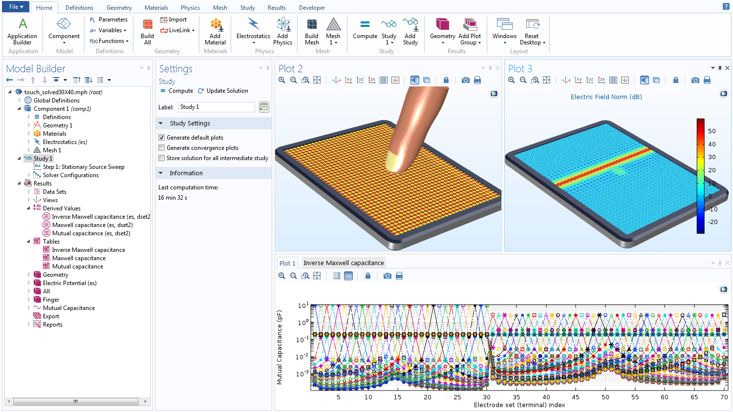
The Touchscreen Simulator application in the AC/DC Module Application Library computes the capacitance matrix of a touchscreen in the presence of a human finger, represented by a phantom. The position and orientation of the finger are controlled via input parameters and the resulting capacitance matrix is evaluated. The image shows the underlying model used to build the Touchscreen Simulator app. The model now uses the Stationary Source Sweep study step, which provides a far faster solution.
Application Library path for an example using the Stationary Source Sweep study step:
ACDC_Module/Applications/touchscreen_simulator
Solver Support for Hybrid BEM/FEM Problems
Sometimes, multiphysics problems can be solved with one numerical method, but are optimally solved using different numerical methods — the boundary element method (BEM) and finite element method (FEM) — for the different physics. Hybrid BEM/FEM models can be used where the matrix storage is the optimal sparse format for the FEM part and a dense or matrix-free format for the BEM part. This makes it possible to use a separate preconditioner/smoother for the individual FEM and BEM parts of the matrix.
It is possible, for example, to use an efficient iterative solver with a hybrid preconditioner. The FEM part can rather freely be preconditioned as usual while the BEM part can be used with one of the aforementioned preconditioners for the near-field matrix. The iterative method computes the residual with a hybrid matrix-based/matrix-free method, making optimal use of different sorts of fast matrix-vector products.
New Tutorial Models: Capacitive Position Sensor (Boundary Elements and Finite Elements)
Two new electrostatic tutorial models in the AC/DC Module Application Library explain how to extract lumped matrices by means of the new Stationary Source Sweep study step, while also showing the benefits of using BEM.
The capacitance matrix of a five-terminal system is computed and used to identify the position of a metallic object. Extra study features and modeling techniques are showcased, such as sweeping on a subset of the terminals. The models also compare how the study’s performance is affected when using direct and iterative solvers.
The tutorial models further compare using FEM with BEM using two different physics interfaces: Electrostatics and Electrostatics, Boundary Elements. When FEM is used, a volumetric mesh of a portion of the surrounding air is necessary; when using BEM, it is not necessary. BEM requires only the meshing of the conductor surfaces and at the interfaces where dielectric properties change.
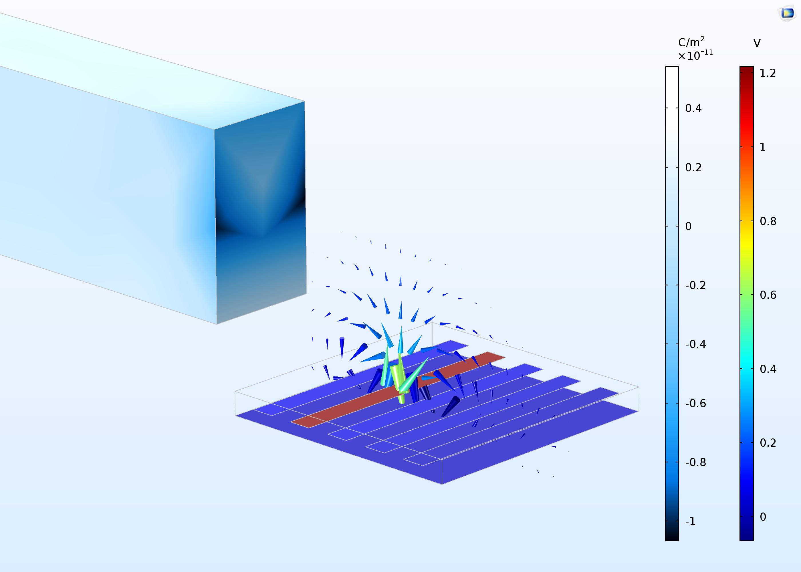
Results from the Capacitive Position Sensor model using the Electrostatics, Boundary Elements interface. The electric field is shown as the arrow direction and size; the electric potential is shown through the arrow and sensor surface color (Rainbow color plot). On the test metal block, the induced surface charge density is plotted (Jupiter Aurora Borealis color plot).
Application Library paths for the Capacitive Position Sensor models:
ACDC_Module/Tutorials/capacitive_position_sensor
ACDC_Module/Tutorials/capacitive_position_sensor_bem
New Tutorial Model: Axisymmetric Approximation of a 3D Inductor
Inductive devices experience capacitative coupling between conductors at high frequencies. Modeling this phenomenon requires that you describe electric fields that have components both parallel with and perpendicular to the wire. This consideration might lead to the conclusion that a 3D model is always necessary to model the phenomenon, even if the coil is a helix, which is actually not the case.
The 3D inductor example demonstrates how to extract information related to the self-resonance of a 3D inductor by means of an axisymmetric simulation. In order to achieve a correct 2D axisymmetric model, an effective axisymmetric core is created, and the RLC Coil Group feature is employed. This lean method is particularly suitable for studying systems with thousands of turns, such as sensors or transformers, thus keeping the computational costs low.
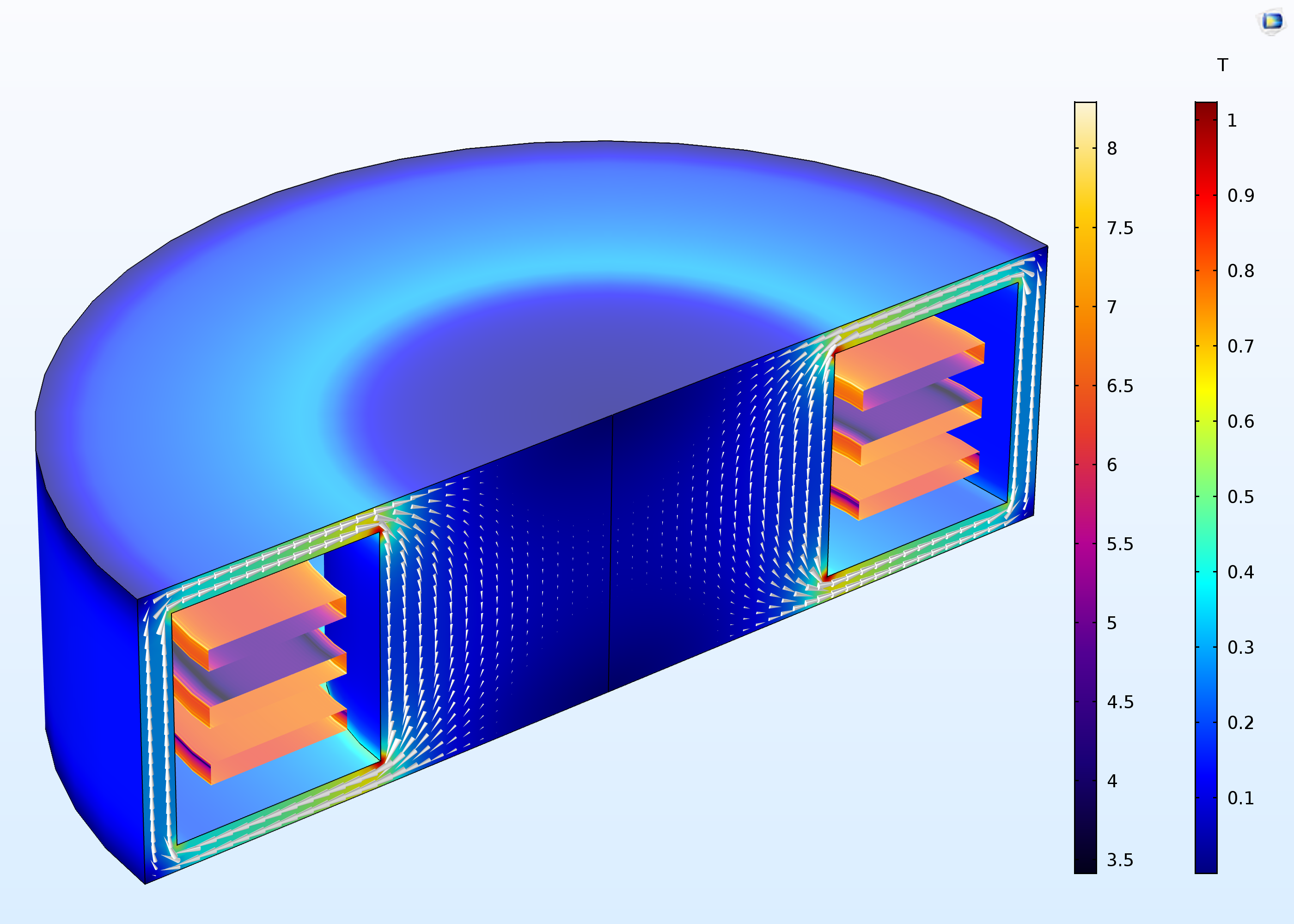 A 3D view of a revolved 2D axisymmetric simulation of an inductor. The simulation shows the results at 6.5 MHz, which is near self-resonance. Shown is the magnetic flux density in the core (Rainbow color plot) and the loss density (in W/m3) on the surface of the winding (Heat Camera color plot). The arrow plot shows the electric field.
Application Library path for the Axisymmetric Approximation of a 3D Inductor model:
ACDC_Module/Inductive_Devices_and_Coils/axisymmetric_approximation_of_inductor_3d
New Tutorial Model: Permanent Magnet Motor in 3D
Permanent magnet (PM) motors are used in many high-end applications, such as in electric and hybrid vehicles, for example. An important design limitation is that the magnets are sensitive to high temperatures, which can occur through heat losses caused by currents — in particular, eddy currents.
Here, an 18-pole PM motor is modeled in 3D to accurately capture eddy current losses in the magnets. The central part of the geometry, containing the rotor and part of the air gap, is modeled as rotating relative to the coordinate system of the stator. Sector symmetry and axial mirror symmetry are leveraged to reduce the computational effort while still capturing the full 3D behavior of the device.
An additional dependent variable is used to compute and store the time integral of the eddy current loss density in the magnets. This could later be used as a distributed, time-averaged heat source in a separate heat transfer analysis, where the thermal time scale is typically much larger than that of the eddy current losses.
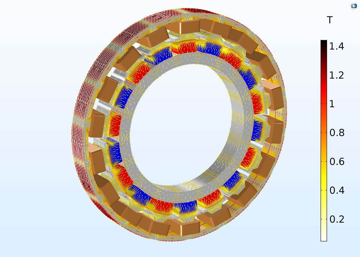
Depiction of the full geometry of the permanent magnet motor with coils (copper); rotor and stator (gray); and permanent magnets (red and blue, depending on the radial magnetization). The magnetic flux density, B, is shown as an arrow plot with its associated color legend.
Animation of the permanent magnet motor with coils (copper); rotor and stator (gray); and permanent magnets (red and blue, depending on the radial magnetization). The magnetic flux density, B, is shown as an arrow plot with its associated color legend.
Animation of a sector cycle showing arrow plots of eddy currents in the magnet (white), magnetic flux density B (Thermal Light color plot), and coil current (gray). The surface plot (Heat Camera color plot) shows the time-averaged eddy current loss density in the magnet.
Application Library path for the Permanent Magnet Motor in 3D model:
ACDC_Module/Motors_and_Actuators/pm_motor_3d
New Tutorial Model: Electrodynamics of a Magnetic Power Switch
Electrical events, such as an overcurrent or overload, can seriously damage electrical circuits or power lines. To avoid expensive replacements of critical parts, electric switch circuit breakers can be installed. These mechanically interrupt the current flow or surge by moving a plunger as soon as a critical current is reached. In contrast to a fuse, which has to be replaced after it has been activated to protect the surrounding electrical components, a circuit breaker can be reset.
The main purpose of this tutorial model is to explore the working principle and some possible solutions for modeling one class of circuit breaker: magnetic power switches. This is an electromechanical device in which iron plungers are moved by means of the magnetic attraction exerted by current flowing in coils surrounding it. Turning off the driving current resets the switch to its initial state.
The model simulates rigid body dynamics under the influence of magnetic forces, induced currents, and spring/constraint arrangements that keep the plunger in its equilibrium position. A copper coil is placed on the central leg of a lower E-core, which is kept fixed. As current flows in the coil, an attractive force is exerted on the upper E-core (the moving plunger), which is held in place by a prestressed spring. When the force reaches a threshold value, the plunger moves toward the lower E-core, closing the air gap. The model illustrates how to properly simulate the movement and the closing time, which depends on the spring stiffness.
Application Library path for the Magnetic Power Switch model:
ACDC_Module/Motors_and_Actuators/power_switch
New Tutorial Model: Operational Amplifier with Capacitive Load
An operational amplifier (op-amp) is a differential voltage amplifier with a wide range of applications in analog electronics. This tutorial models an op-amp connected to a feedback loop and a capacitive load.
The op-amp is modeled as an equivalent linear subcircuit in the Electrical Circuit interface where it is inserted into an outer circuit. The model is partially based on the SPICE format. The model is simulated for 10 ms with data output every 0.05 ms. The internal dynamics of the op-amp interact with the feedback network, causing ringing in the output signal (step response).
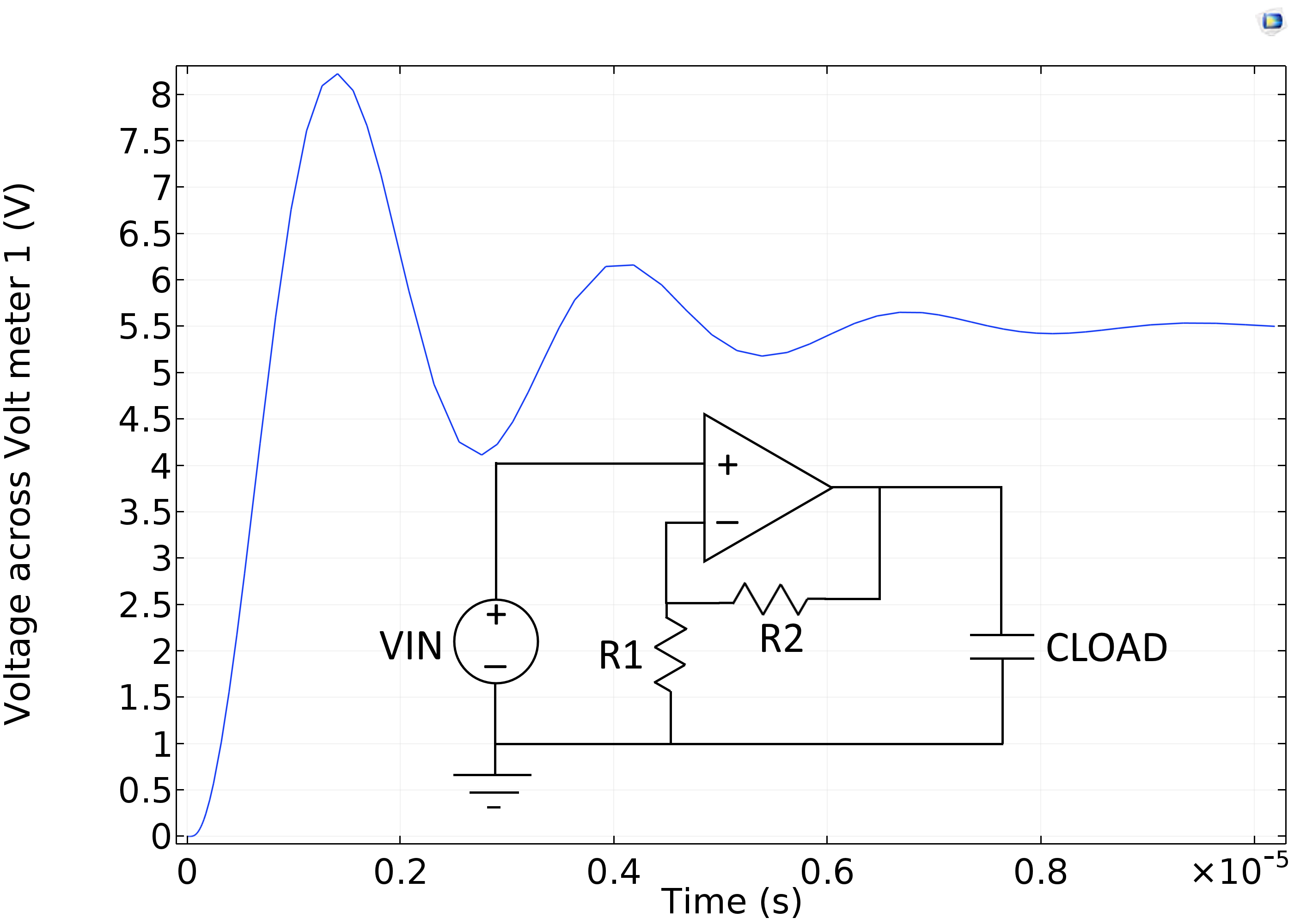 The output voltage across the load capacitor is measured for a step voltage input of 0.5 V. The measured voltage across the load capacitor exhibits damped oscillations.
Application Library path for the Operational Amplifier with Capacitive Load model:
ACDC_Module/Tutorials/opamp_capacitive_load
New Tutorial Models: Cable Tutorial Series
A new set of tutorials consisting of six models and associated documentation investigates the capacitive, inductive, and thermal properties of a standard three-core lead-sheathed XLPE HVAC (cross-linked polyethylene, high-voltage alternating current) submarine cable (500 mm2, 220 kV). The series is intended both for experts looking to get up to speed on how to model such applications in COMSOL Multiphysics® and for students and engineers interested in the electromagnetic phenomena associated with cables and how they can be modeled.
The series starts by going over the fundamental principles of the physics involved and then increases in complexity based on additional physical factors and behavior that could be considered. Apart from discussing electromagnetic modeling in relation to cables — such as charging currents, bonding types, armor twists, and temperature dependency — a lot of attention is also given to modeling electromagnetism and the methods involved.
 A three-core lead-sheathed cable is modeled considering its environment surrounded by earth. The temperature distribution inside the cable is shown as a 3D color plot above geometry.
Application Gallery link: Cable Tutorial Series
Application Library path for the models in the Cable Tutorial Series:
ACDC_Module/Tutorials,Cables/submarine_cable_01_introduction
ACDC_Module/Tutorials,Cables/submarine_cable_02_capacitive_effects
ACDC_Module/Tutorials,Cables/submarine_cable_03_bonding_capacitive
ACDC_Module/Tutorials,Cables/submarine_cable_04_inductive_effects
ACDC_Module/Tutorials,Cables/submarine_cable_05_bonding_inductive
ACDC_Module/Tutorials,Cables/submarine_cable_06_thermal_effects