Wave Optics Module Updates
For users of the Wave Optics Module, COMSOL Multiphysics® version 6.0 brings a new Part Library for slab and rectangular waveguide elements, three new tutorial models, and an Electromagnetic Waves, Boundary Elements interface. Read more about these updates below.
Electromagnetic Wave, Boundary Elements
When modeling the scattering properties of objects, evaluating electric fields far from the scatterer, or far-fields of an antenna placed on an electrically large platform, the formulation based on the boundary element method (BEM) can improve the computation efficiency. The new physics interface called Electromagnetic Waves, Boundary Elements solves the vector Helmholtz equation for piecewise-constant material properties with the electric field as the dependent variable. The boundary element method (BEM) can be coupled to the finite element method (FEM), so-called hybrid BEM–FEM, to compute the field and interaction with other conductive objects outside the FEM domains.
Part Library for Slab and Rectangular Waveguide Elements
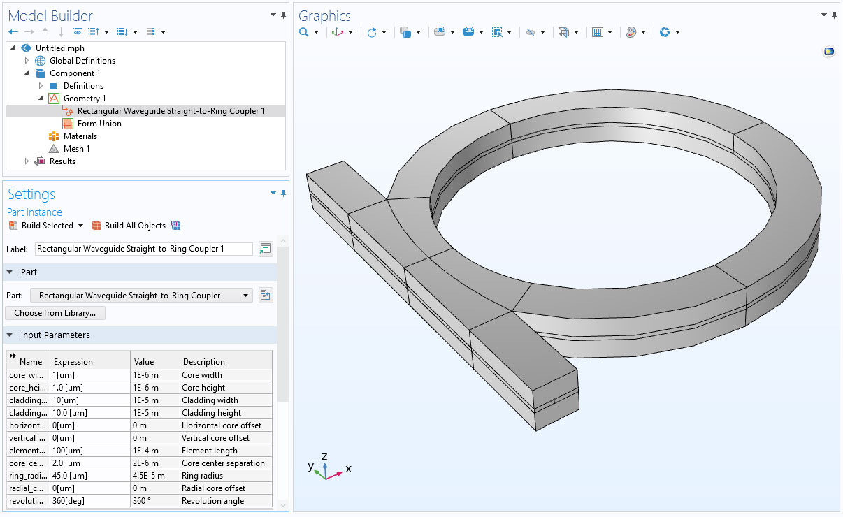
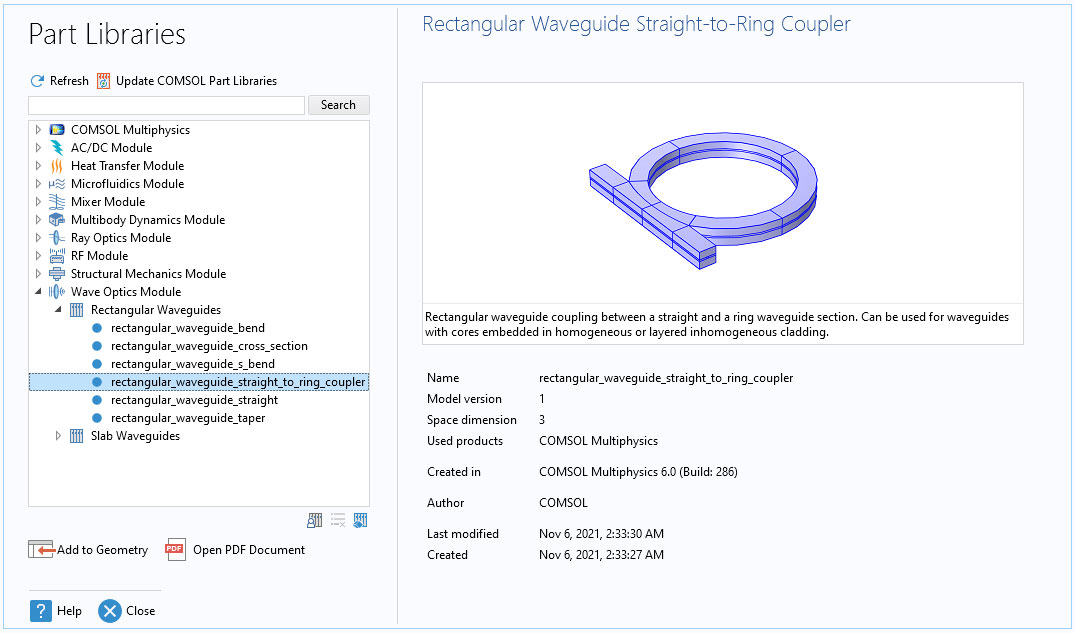
The new Wave Optics Module Part Library for slab and rectangular waveguide elements simplifies the construction of complex waveguide structures. The library includes parts for the following waveguide elements:
- Straight waveguides
- Tapered waveguides
- Bent (ring) waveguides
- S-bend waveguides
- Couplers
These parts are fully parameterized and include predefined selections for material domain selections, physics feature selections, and to simplify mesh generation. The Mach Zehnder Modulator model is now built using S-bend Directional Coupler and Straight Waveguide parts, which makes it easy to define the material domains, the physics feature selections, and the mesh. The Optical Ring Resonator Notch Filter model is now built using a Straight-to-Ring Coupler part, which makes it easy to use a mapped mesh.
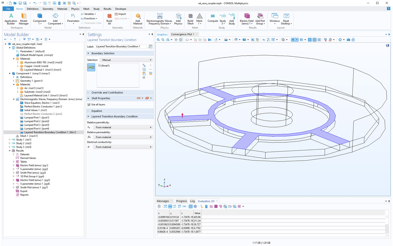
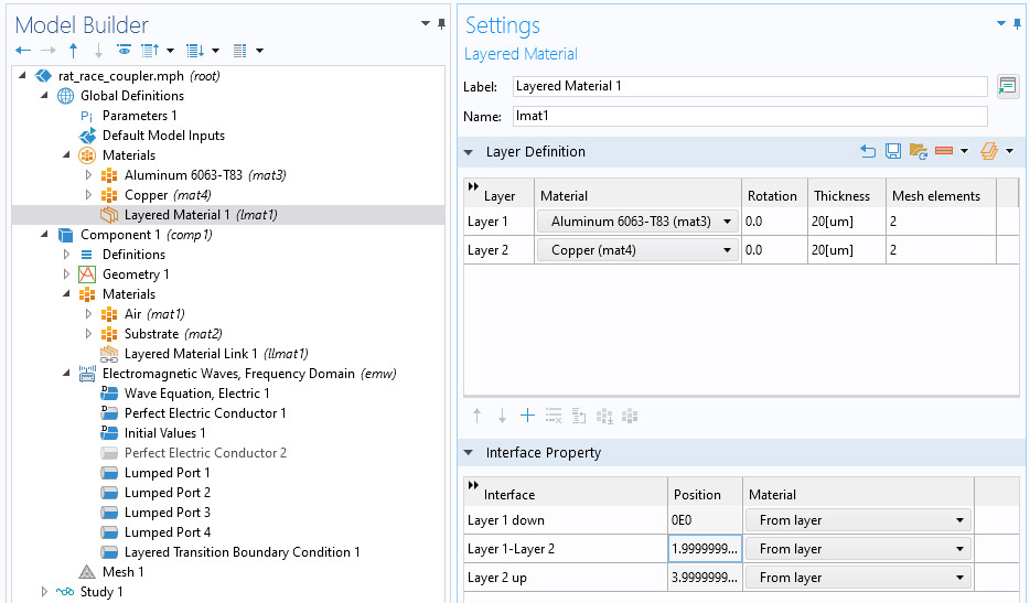
Layered Transition Boundary Condition
Multiple thin layers, such as the gold-plated copper of a circuit board trace or close-to-normal incidence on an antireflection coating to an optical lens, can be described by the new Layered Transition Boundary Condition feature. It requires combining this boundary condition with the Layered Material feature in the global Materials, and Layered Material Link feature in the component Materials node. You can see this new feature demonstrated in the Rat-Race Coupler tutorial model.
New Tutorial Models
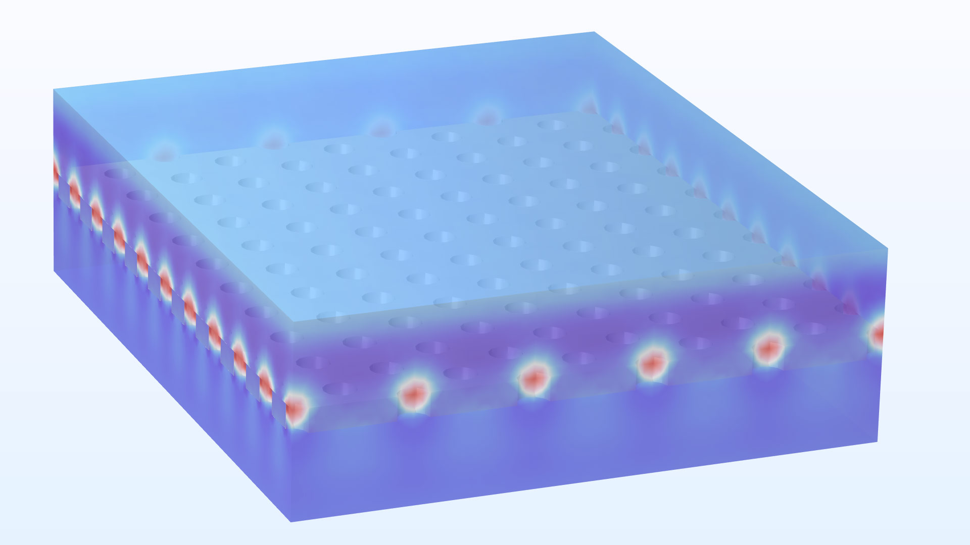
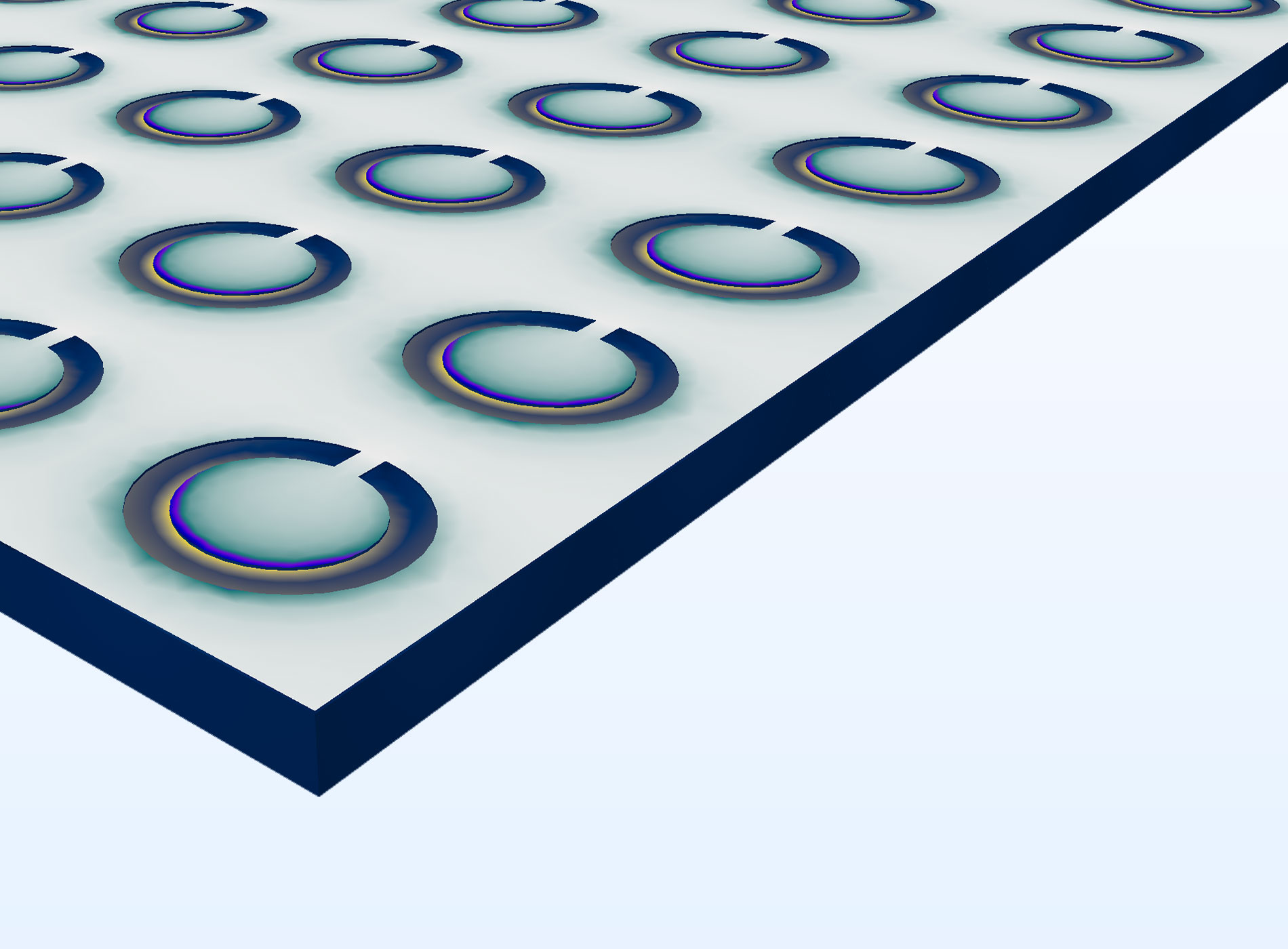
Hexagonal Plasmonic Color Filter
The Hexagonal Plasmonic Color Filter tutorial model demonstrates how to perform simulations of an absorbing bandstop color filter, based on a hexagonal array of holes in a thin aluminum layer. While the structure is hexagonally periodic, this example also shows how to set the model up as rectangularly periodic. This makes it easier to use array datasets to plot the results from several unit cells. However, since the rectangular unit cell is larger than the hexagonal unit cell, there is more memory consumption and longer solution time.
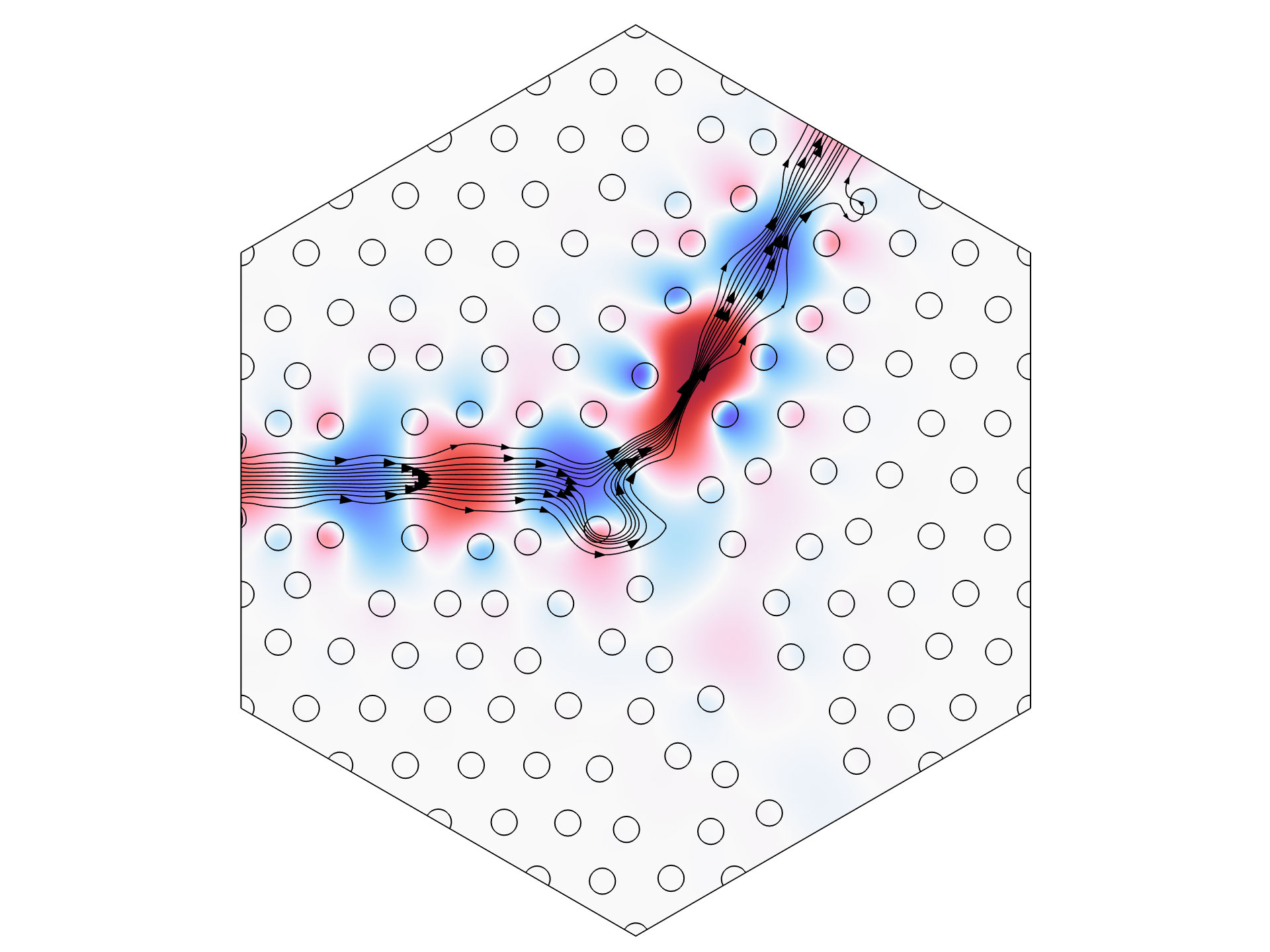
Optimization of a Photonic Crystal for Demultiplexing
The Optimization of a Photonic Crystal for Demultiplexing tutorial model, published with COMSOL Multiphysics® version 5.6, has been updated to include a new hexagonal geometry. The objective is to maximize the output power ratio between two narrow frequency bands while constraining the losses from below, achieved by letting GaAs pillars change position but not shape.
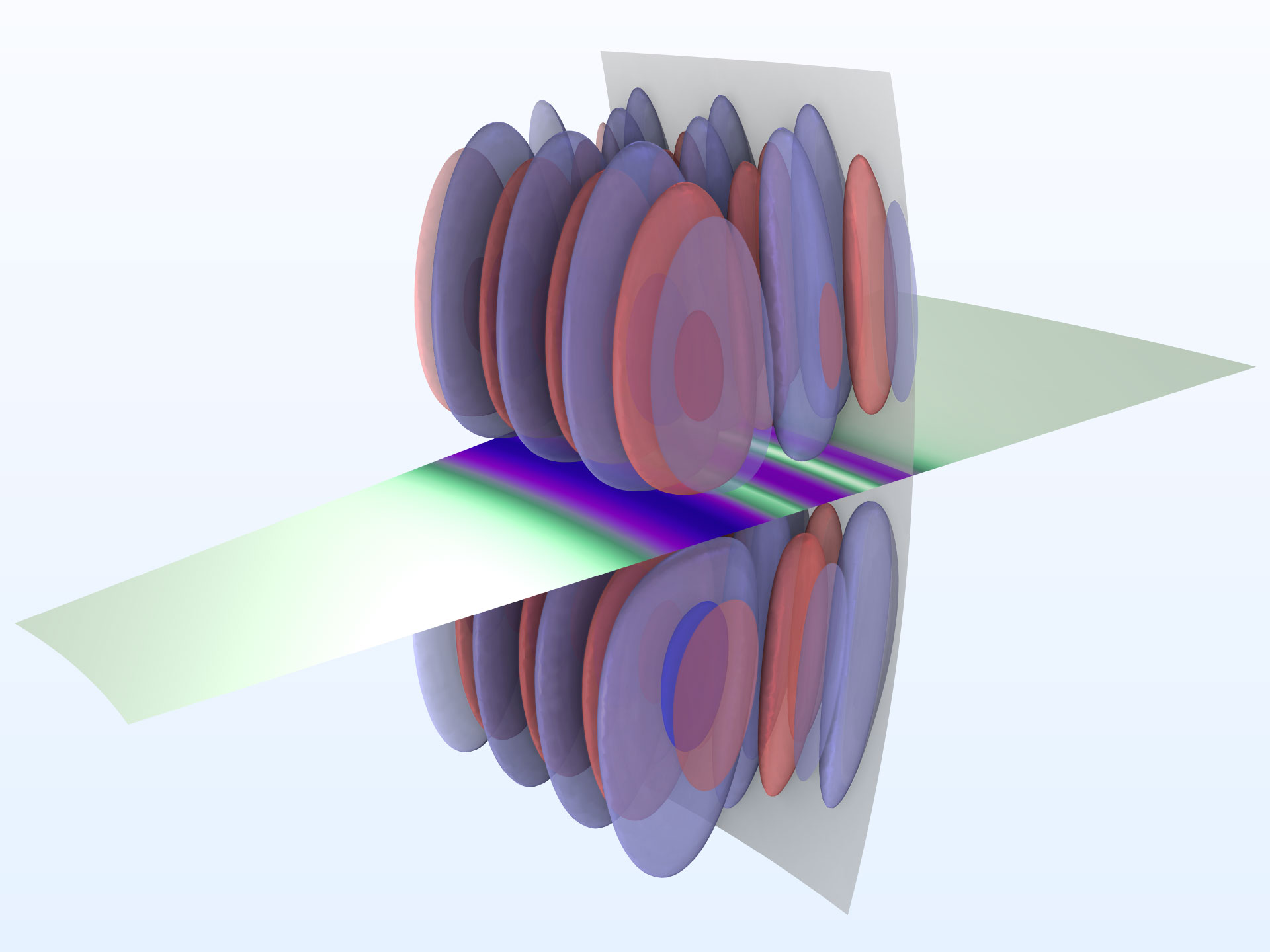
Whispering Gallery Mode Resonator
The Whispering Gallery Mode Resonator tutorial model shows how to compute the different eigenmodes and resonance frequencies of a whispering gallery mode resonator with high optical quality factors. The resonance frequencies are filtered in two ways: by their spatial localization in the resonator or by comparing the losses of the bound modes and the air modes (undesired, in this case).
Optical Material Library Improvements
In the Optical material library, available for the Ray Optics Module and Wave Optics Module, glasses from SCHOTT AG, CDGM Glass Company Ltd., Ohara Corporation, and Corning Inc. are now presented with more comprehensive material data. In addition to optical dispersion coefficients and thermo-optic coefficients, many of these glasses now include internal transmittance, density, Young's modulus, Poisson's ratio, coefficient of linear thermal expansion, thermal conductivity, and specific heat capacity. With the inclusion of more comprehensive material data for optical glasses, it is now easier than ever to set up coupled structural-thermal-optical performance (STOP) analysis models.
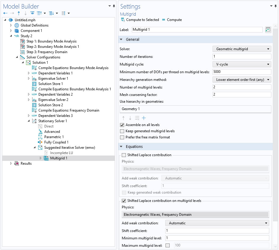
Shifted Laplace Contribution on Multigrid Levels
If no geometrical feature sizes are smaller than half a wavelength and the operating frequency is high, modeling with a higher-order element such as cubic element discretization is beneficial for faster computation. The computation efficiency can be further improved by selecting the Shifted Laplace contribution on multigrid levels check box under the Multigrid study settings.
Smoothed Heat Source Calculation
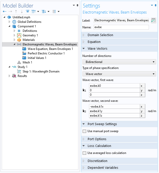
In the bidirectional formulation for the Electromagnetic Waves, Beam Envelopes interface, a new Use an averaged loss calculation option is available to remove cross terms between the two waves that are not resolved by the mesh. If this spatially fast varying heat source distribution is in any way washed out by the heat transfer, it can be advantageous to exclude the cross terms when calculating the electromagnetic loss (and heat source).
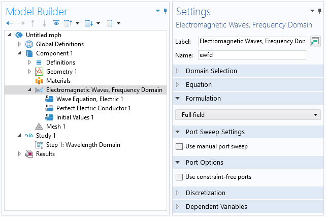
Constraint-Free Port Formulation
The Use constraint-free ports option is available to calculate the expansion coefficients as overlap integral, while in the default port formulation, the expansion coefficients (or S-parameters) are calculated by adding a scalar dependent variable for each coefficient and then adding a constraint to enforce the series expansion. This new option can be advantageous when using many ports, as no constraint elimination is required.
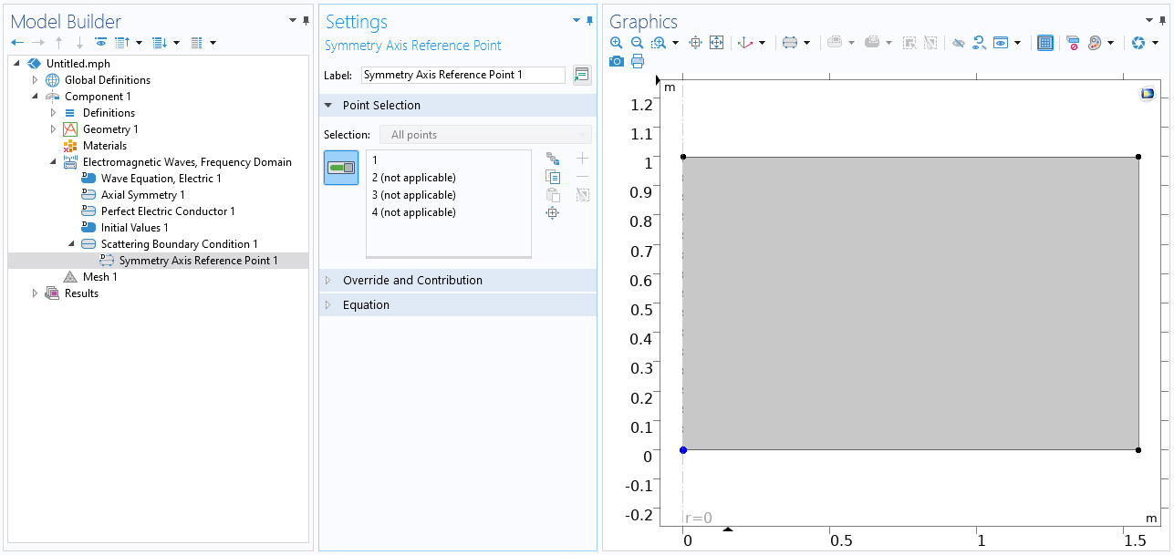
Symmetry Axis Reference Point
A new Symmetry Axis Reference Point feature helps to define Gaussian beam input fields in 2D axisymmetry. In the Scattering Boundary Condition or Matched Boundary Condition nodes, this is added as a default subnode when an incident field is defined. The Symmetry Axis Reference Point feature defines a reference position at the intersection point between the parent node's boundary selection and the symmetry axis.
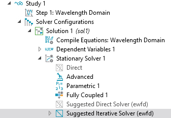
Iterative Solver Suggestion for Periodic Structures
Typical periodic problems are solved with a direct solver. However, the direct solver consumes a lot of memory when the periodic unit cell size is not subwavelength. In this case, switch to the Suggested Iterative Solver to finish the computation faster with less memory usage.
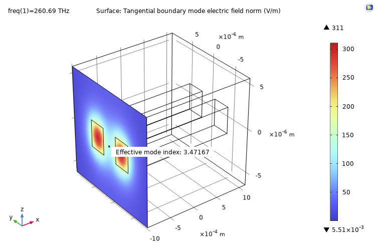
Default Plots for Numeric Port Mode Fields
To simplify the inspection of the port mode fields, they are now automatically created when Numeric port types are used. You can see this default plot in the updated Directional Coupler and Optical Ring Resonator Notch Filter tutorial models.