RF Module Updates
For users of the RF Module, COMSOL Multiphysics® version 5.4 brings additional far-field functionality and variables for efficient antenna and radiation pattern analysis, an extended material library for microwave and millimeter-wave circuit boards, and enhanced Application Library examples with more visualization effects and deployment of commercially available connectors from the RF Part Library. Browse all of the RF Module updates in more detail below.
Uniform Antenna Array Factor Function
It is now possible to evaluate the radiation pattern of an antenna array very quickly from the radiation pattern of a single antenna element by using an asymptotic approach that multiplies the far field of a single antenna with a uniform array factor. You can find this functionality in the updated Microstrip Patch Antenna model.
An 8x8 microstrip patch antenna array pattern synthesized from a single microstrip antenna simulation.
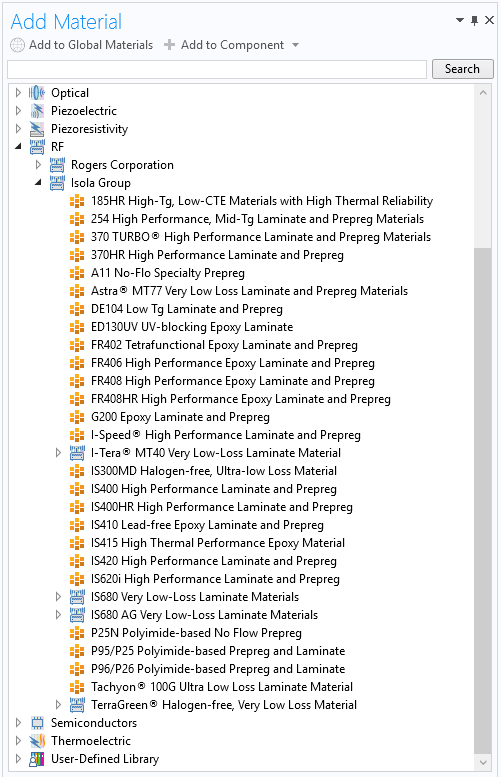
Additional RF Material Library for Substrates
The RF Module enhances its material library with more than 40 substrate materials from the company Isola Group to assist in modeling printed RF, microwave, and millimeter-wave circuits. The RF Module material library now provides more than 100 substrate materials.
3D Far-Field and RCS Functions from 2D Axisymmetric Models
By utilizing new far-field functions, a 2D axisymmetric model is now more useful for the purpose of quick estimation of the far-field response of the equivalent 3D model. A set of 3D far-field norm functions are available in a 2D axisymmetric geometry for the following cases:
- Antenna models using circular port excitation with a positive azimuthal mode number
- Scattered field analysis excited by the predefined circularly polarized plane wave type
Far-Field Norm Functions
| Description | Name | Full Name Examples | Full Name Description |
|---|---|---|---|
| 3D far-field norm | norm3DEfar | norm3DEfar_TE12 | Azimuthal mode number 1, TE mode circular port with mode number 2 |
| 3D far-field norm, dB | normdB3DEfar | normdB3DEfar_TM21 | Azimuthal mode number 2, TM mode circular port with mode number 1 |
More Far-Field Postprocessing Variables
New variables for computing the maximum directivity, gain, and realized gain have been added. These variables are available for global evaluation, without plotting a 3D far-field pattern. They can be accessed when the selection for the far-field calculation feature is spherical (in 3D) and circular (in 2D axisymmetry) and when the center is at the origin.
Far-Field Postprocessing Variables
| Description | Name | Available Component |
|---|---|---|
| Maximum directivity | maxD | 2D Axisymmetric, 3D |
| Maximum directivity, dB | maxDdB | 2D Axisymmetric, 3D |
| Maximum gain | maxGain | 2D Axisymmetric, 3D |
| Maximum gain, dB | maxGaindB | 2D Axisymmetric, 3D |
| Maximum realized gain | maxRGain | 2D Axisymmetric, 3D |
| Maximum realized gain, dB | maxRGaindB | 2D Axisymmetric, 3D |
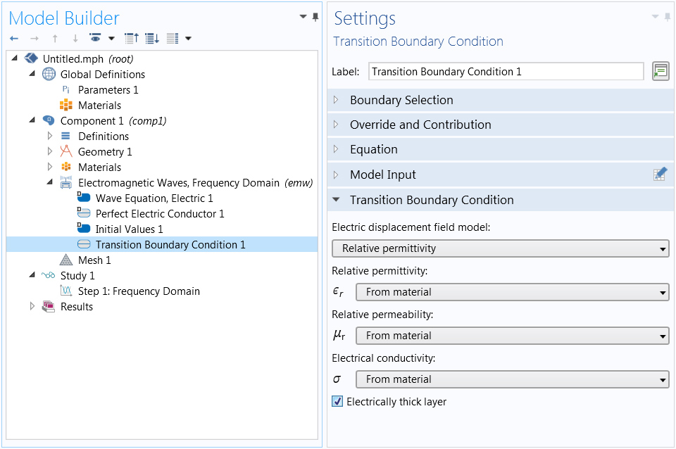
Electrically Thick Layer in Transition Boundary Conditions
The new Electrically thick layer option decouples the two domains that are adjacent to a transition boundary condition. The boundary performs like an interior impedance boundary condition, but the layer geometry can be a surface rather than a domain.
Time-Domain Bandpass Impulse Response via FFT
While transient analyses are useful for time-domain reflectometry (TDR) to handle signal integrity (SI) problems, many RF and microwave examples are addressed using frequency-domain simulations that generate S-parameters. By performing the frequency-to-time fast Fourier transform (FFT) after the conventional frequency domain study, TDR analysis is feasible. This type of analysis helps in identifying physical discontinuities and impedance mismatches on a transmission line by investigating the signal fluctuation in the time domain. You can see this functionality in the new Study of a Defective Microstrip Line via Frequency-to-Time FFT Analysis model.
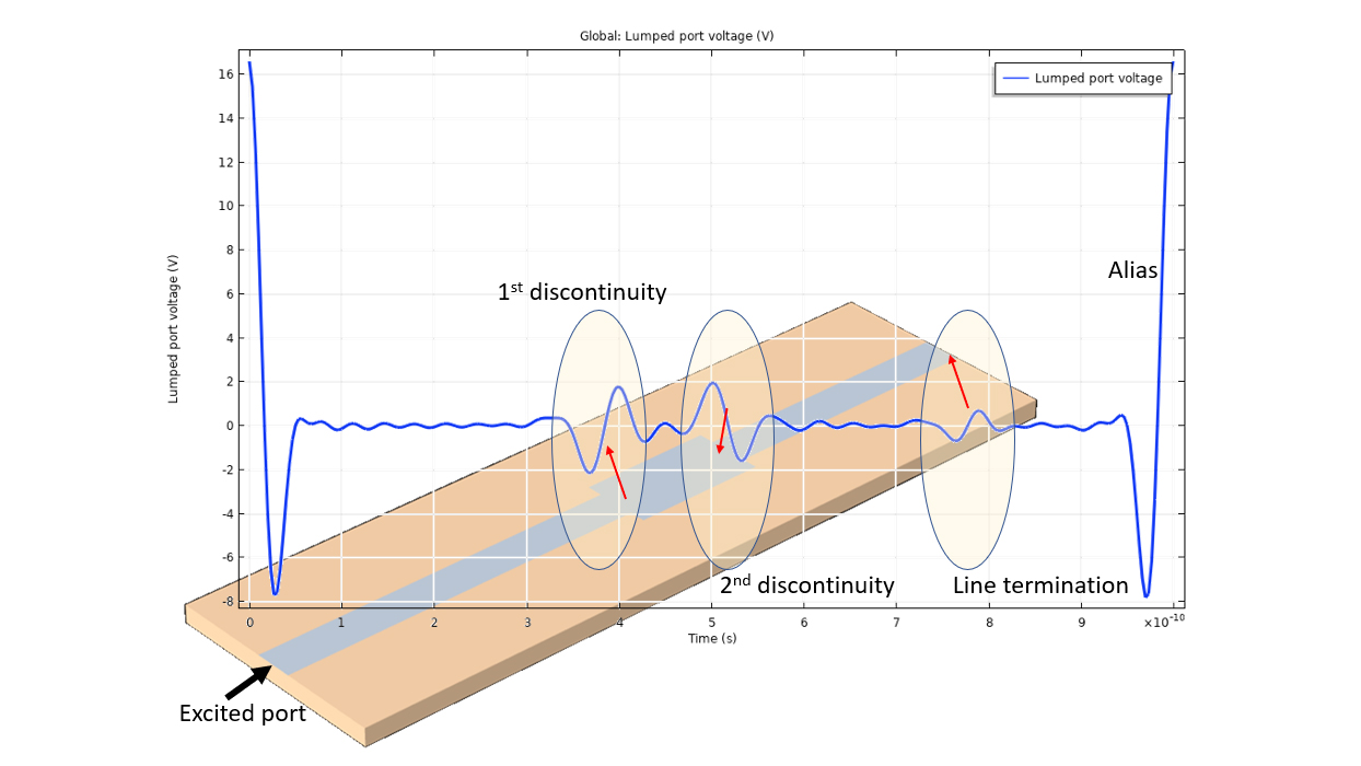 An example where a time-domain lumped port voltage is used. The overshoot and undershoot of the signal are due to the discontinuities of the microstrip line.
Far-Field Analysis in a Transient Study
A far-field domain calculation feature is now available with the Electromagnetic Wave, Transient interface. Using this feature, you can perform a frequency-domain wideband antenna far-field pattern analysis by first running a transient response analysis, followed by a time-to-frequency FFT. You can see this functionality demonstrated in the new Transient Analysis of a Printed Dual-Band Strip Antenna model.
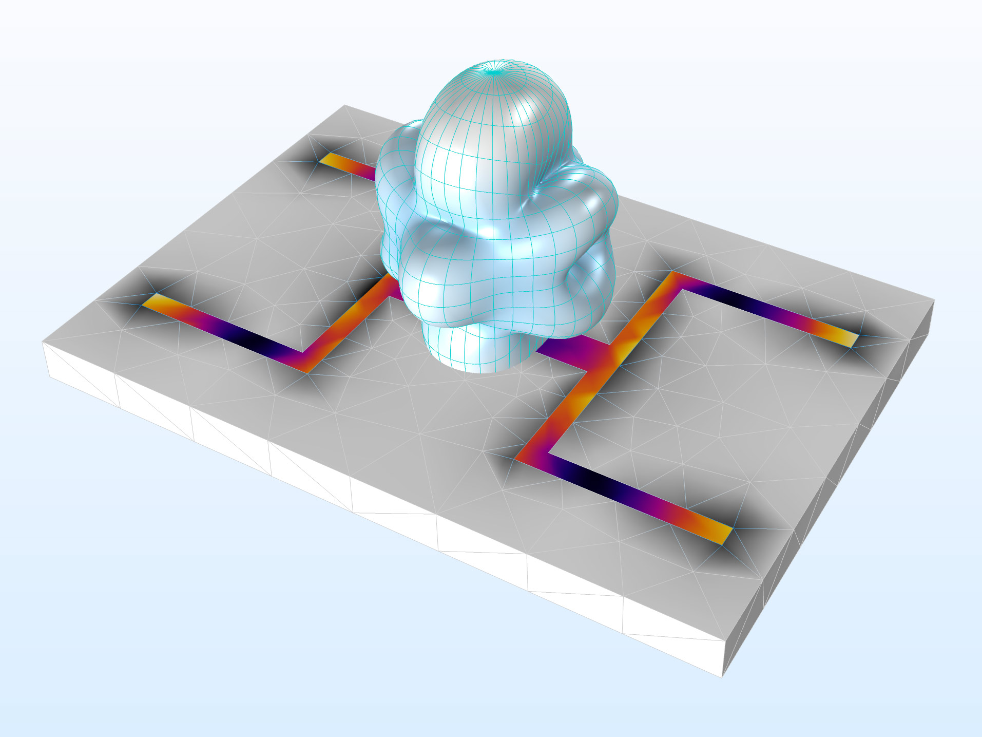 A printed dual-band antenna strip with a visualization of the far-field radiation pattern at the second resonance. The electric field norm distribution at the top of the dielectric board is also shown.
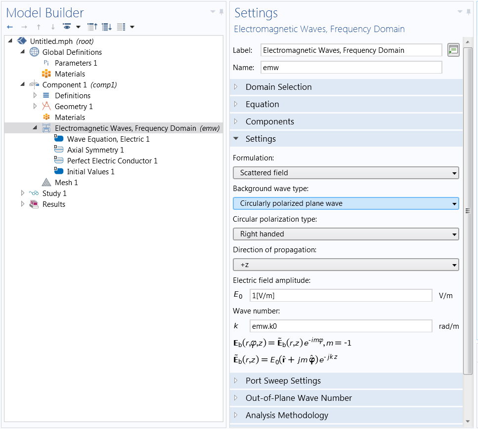
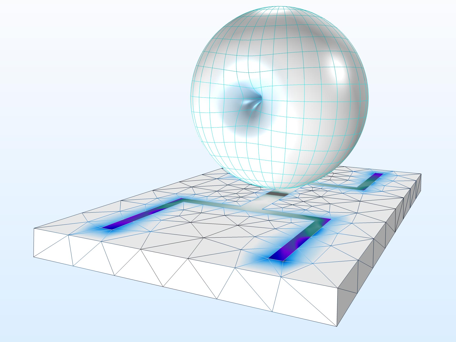
Circularly Polarized Background Field for 2D Axisymmetry
A Circularly polarized plane wave option is now available for the scattered field formulation when modeling with a 2D axisymmetric component. To use this functionality, start by exciting an axisymmetric scatterer with a circularly polarized background field in a 2D axisymmetric model. Then, by using the norm3DEfar function, estimate the far field and radar cross section (RCS) of the same scatterer in 3D, illuminated by a linearly polarized background field.
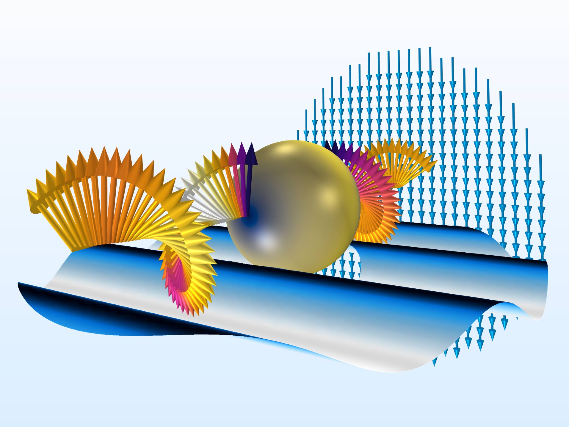 A 3D representation of a 2D axisymmetric model. The scattered field response of a 3D sphere, excited by a linearly polarized background field, can be estimated quickly by a 2D axisymmetric model with a circularly polarized background field.
Improved User Experience for Defining Ports
In- and Outport Direction
Arrow indicators now help to quickly identify which ports are inports (excitations) and which are outports (listeners). The arrow points in the direction of the power flow. An excited port is indicated by an inward arrow on the port boundary, while a listener port has an outward arrow. Lumped ports also support this visualization feature.
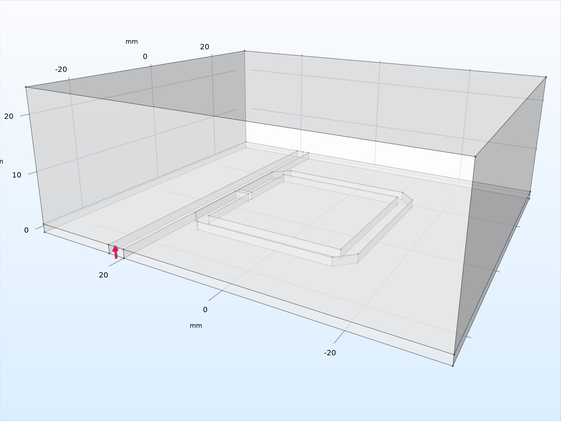
 For the excited port boundary in this example model of an iris filter waveguide, the direction of power flow is shown as a red arrow.
Numeric TEM Ports with Voltage Drop Direction
When numeric ports are analyzed by means of a boundary mode analysis, degenerated modes are challenging to handle with respect to S-parameter calculations. For better handling of such cases, the voltage drop direction is now indicated by a red arrow tangential to the port boundary, and fixes the port mode field polarization. The direction can be changed by checking the Toggle Voltage Drop Direction box in the Settings window of the Integration Line for Voltage node, which is a subfeature of the numeric TEM port feature. You can see this functionality used in the updated Notch Filter Using a Split Ring Resonator model.
 The voltage drop direction for a numeric TEM port is indicated with a red arrow.
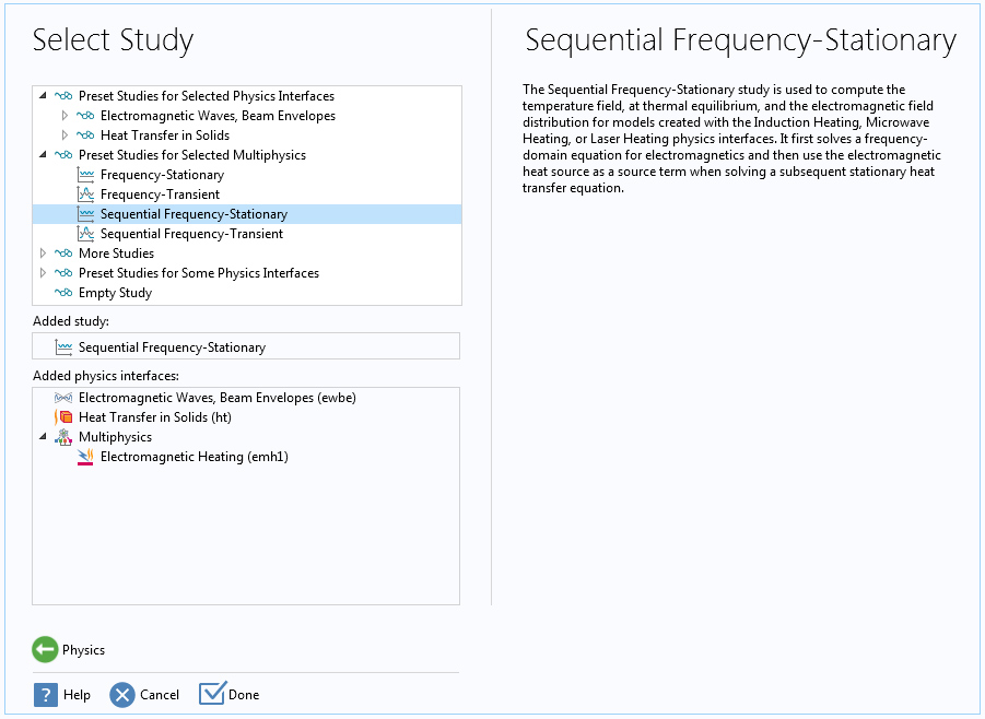
One-Way Coupled Multiphysics in the Model Wizard
For multiphysics involving electromagnetic heating, such as Laser Heating in the Wave Optics Module or Microwave Heating in the RF Module, there are now two new study sequences available in the Model Wizard. The Sequential Frequency-Stationary study first solves a frequency-domain equation for electromagnetics and then uses the electromagnetic heat source as a source term when solving a subsequent stationary heat transfer equation. The Sequential Frequency-Transient study first solves a frequency-domain equation for electromagnetics and then uses the electromagnetic heat source as a source term when solving a subsequent time-dependent heat transfer equation. For both study sequences, it is assumed that the electromagnetics analysis does not depend on the computed temperature distribution. Whenever this simplifying assumption can be made, solving the two physics in a sequence requires fewer computational resources.
You can see this functionality used in the following models:
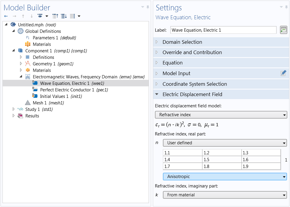
Fully Anisotropic Refractive Index
When the Refractive index option is selected for the Electric displacement field model combo box in wave equation features, you can now input a fully anisotropic tensor. A matrix-matrix multiplication is used to transform this refractive index tensor to the relative permittivity tensor.
Important Enhancements
- Perfect electric conductor (PEC), perfect magnetic conductor (PMC), and surface current density can now be applied to interior boundaries, when using the Electromagnetic Waves, Time Explicit interface
- A new Lumped port option is available in the Electromagnetic Waves, Time Explicit interface for calculating S-parameters at ports located on exterior boundaries
- Several tutorial models use commercially available SMA connectors from the RF Part Library, providing more realistic and accurate simulations:
- To improve legibility of the default black text appearing on parts of plots with lower numerical values, the default color table has been changed to RainbowLight
- Several tutorial models in the Application Library have been updated to showcase additional visualization features:
- biconical_frame_antenna (Isosurface plot)
- dipole_antenna (Isosurface plot)
- helical_antenna (Axial ratio plot, Isosurface plot)
- log_periodic_antenna (Isosurface plot)
- vivaldi_antenna (Isosurface plot)
- airplane_antenna_crosstalk (Isosurface plot)
- cascaded_cavity_filter (Isosurface plot)
- cylindrical_cavity_filter_evanescent (Isosurface plot)
- sar_in_human_head (Visualization of a material property)
New Tutorial Models
COMSOL Multiphysics® version 5.4 brings two new tutorial models.
Study of a Defective Microstrip Line via Frequency-to-Time FFT Analysis
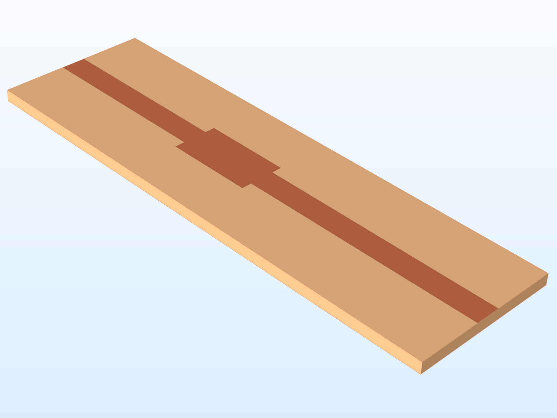 A defective microstrip line circuit board. This tutorial answers the question: Can the discontinuities be detected by simulation?
Search in the Application Library:
microstrip_line_discontinuity
Transient Analysis of a Printed Dual-Band Strip Antenna
 A printed dual-band antenna strip with its far-field radiation pattern at the first resonance. The electric field norm distribution at the top of the dielectric board is also visualized.
Search in the Application Library:
dual_band_antenna_transient